This tutorial is divided into the following sections:
This tutorial illustrates the setup and solution of a three-dimensional turbulent fluid flow and heat transfer problem in a mixing elbow. The mixing elbow configuration is encountered in piping systems in power plants and process industries. It is often important to predict the flow field and temperature field in the area of the mixing region in order to properly design the junction.
This tutorial demonstrates how to do the following:
Use the Watertight Geometry guided workflow to:
Import a CAD geometry
Generate a surface mesh
Describe the geometry
Generate a volume mesh
Launch Ansys Fluent.
Read an existing mesh file into Ansys Fluent.
Use mixed units to define the geometry and fluid properties.
Set material properties and boundary conditions for a turbulent forced-convection problem.
Create a surface report definition and use it as a convergence criterion.
Calculate a solution using the pressure-based solver.
Visually examine the flow and temperature fields using the postprocessing tools available in Ansys Fluent.
Change the solver method to coupled in order to increase the convergence speed.
Adapt the mesh based on the temperature gradient to further improve the prediction of the temperature field.
This tutorial assumes that you have little or no experience with Ansys Fluent, and so each step will be explicitly described.
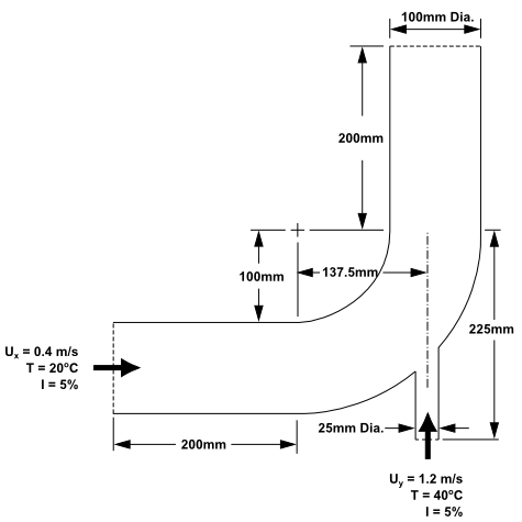
The problem to be considered is shown schematically in Figure 5.1: Problem Specification. A cold fluid at 20° C flows into the pipe through a large inlet, and mixes with a warmer fluid at 40° C that enters through a smaller inlet located at the elbow. The pipe dimensions are in inches and the fluid properties and boundary conditions are given in SI units. The Reynolds number for the flow at the larger inlet is 50,800, so a turbulent flow model will be required.
Note: Since the geometry of the mixing elbow is symmetric, only half of the elbow must be modeled in Ansys Fluent.
To help you quickly identify graphical user interface items at a glance and guide you through the steps of setting up and running your simulation, the Ansys Fluent Tutorial Guide uses several type styles and mini flow charts. See Typographical Conventions Used In This Manual for detailed information.
The following sections describe the setup and solution steps for running this tutorial in serial:
Download the
introduction.zipfile here .Unzip
introduction.zipto your working directory.The SpaceClaim CAD file
elbow.scdoccan be found in the folder. In addition, theelbow.pmdbfile is available for use on the Linux platform.Use the Fluent Launcher to start Ansys Fluent.
Select Meshing in the top-left selection list to start Fluent in Meshing Mode.
Enable Double Precision under Options.
Set Meshing Processes and Solver Processes to
4under Parallel (Local Machine).
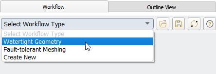
Start the meshing workflow.
In the Workflow tab, select the Watertight Geometry workflow.
Review the tasks of the workflow.
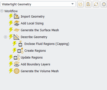
Each task is designated with an icon indicating its state (for example, as complete, incomplete, etc. All tasks are initially incomplete and you proceed through the workflow completing all tasks. Additional tasks are also available for the workflow.
Import the CAD geometry (
elbow.scdoc).Select the Import Geometry task.
For Units, select in from the drop-down list.
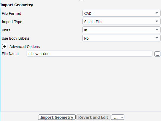
For File Name, enter the path and file name for the CAD geometry that you want to import (
elbow.scdoc).Note: The workflow only supports
*.scdoc(SpaceClaim), Workbench (.agdb), and the intermediary*.pmdbfile formats.Select .
This will update the task, display the geometry in the graphics window, and allow you to proceed onto the next task in the workflow.
Note: Alternatively, you can use the ... button next to File Name to locate the CAD geometry file, after which, the Import Geometry task automatically updates, displaying the geometry in the graphics window, and the workflow automatically progresses to the next task.
Throughout the workflow, you are able to return to a task and change its settings using either the Edit button, or the Revert and Edit button.
Add local sizing.
In the Add Local Sizing task, you are prompted as to whether or not you would like to add local sizing controls to the faceted geometry.
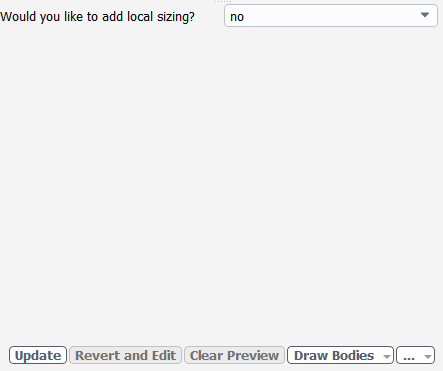
For the purposes of this tutorial, you can keep the default setting of no.
Click Update to complete this task and proceed to the next task in the workflow.
Generate the surface mesh.
In the Generate the Surface Mesh task, you can set various properties of the surface mesh for the faceted geometry.
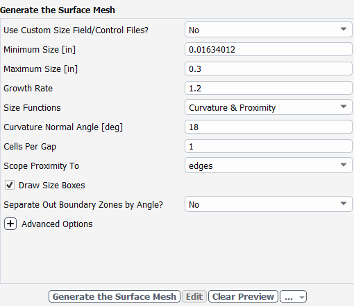
Specify
0.3for Maximum Size.Note: The red boxes displayed on the geometry in the graphics window are a graphical representation of size settings. These boxes change size as the values change, and they can be hidden by using the Clear Preview button.
Click Generate the Surface Mesh to complete this task and proceed to the next task in the workflow.
Describe the geometry.
When you select the Describe Geometry task, you are prompted with questions relating to the nature of the imported geometry.
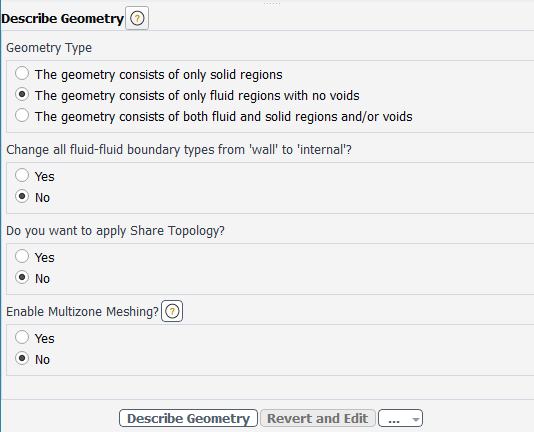
Since the geometry defined the fluid region. Select The geometry consists of only fluid regions with no voids for Geometry Type.
Click Describe Geometry to complete this task and proceed to the next task in the workflow.
Update Boundaries Task
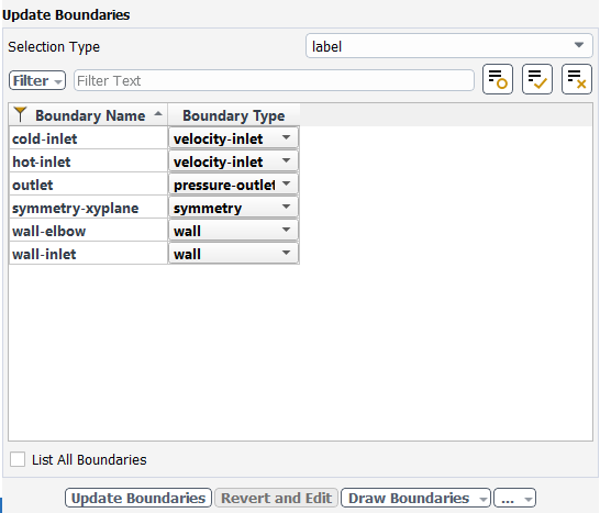
For the Selection Type field, select label.
For the
wall-inletboundary, change the Boundary Type field to wall.Click Update Boundaries to complete this task and proceed to the next task in the workflow.
Update your regions.
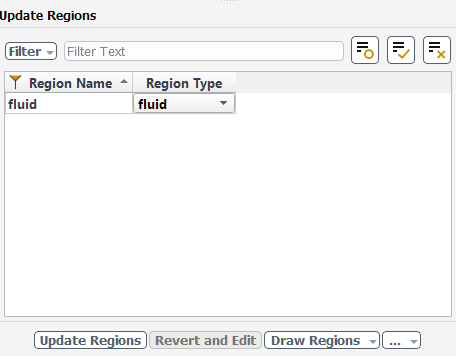
Select the Update Regions task, where you can review the names and types of the various regions that have been generated from your imported geometry, and change them as needed.
Keep the default settings, and click Update Regions.
Add Boundary Layers.
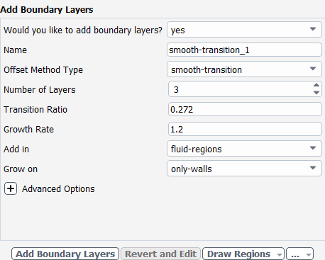
Select the Add Boundary Layers task, where you can set properties of the boundary layer mesh.
Keep the default settings, and click Add Boundary Layers.
Generate the volume mesh.
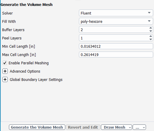
Select the Generate the Volume Mesh task, where you can set properties of the volume mesh.
Select the poly-hexcore for Fill With.
Click Generate the Volume Mesh.
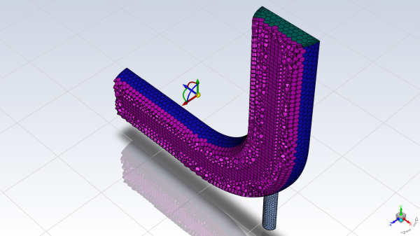
Ansys Fluent will apply your settings and proceed to generate a volume mesh for the manifold geometry. Once complete, the mesh is displayed in the graphics window and a clipping plane is automatically inserted with a layer of cells drawn so that you can quickly see the details of the volume mesh.
Check the mesh.
 Mesh
→ Check → Perform Mesh
Check
Mesh
→ Check → Perform Mesh
Check
Save the mesh file (
elbow.msh.h5). File → Write →
Mesh...
Switch to Solution mode.
Now that a high-quality mesh has been generated using Ansys Fluent in meshing mode, you can now switch to solver mode to complete the set up of the simulation.
We have just checked the mesh, so select Yes when prompted to switch to solution mode.
In this step, you will perform the mesh-related activities using the Domain ribbon tab (Mesh group box).
Check the mesh.
Domain → Mesh
→ Check → Perform Mesh
Check
Ansys Fluent will report the results of the mesh check in the console.
  Domain Extents:
   x-coordinate: min (m) = -2.000000e-01, max (m) = 2.000000e-01
   y-coordinate: min (m) = -2.250000e-01, max (m) = 2.000000e-01
   z-coordinate: min (m) = 0.000000e+00, max (m) = 4.992264e-02
 Volume statistics:
   minimum volume (m3): 1.541854e-11
   maximum volume (m3): 5.483098e-07
     total volume (m3): 2.500657e-03
 Face area statistics:
   minimum face area (m2): 3.010069e-08
   maximum face area (m2): 7.873946e-05
 Checking mesh.....................................
Done.
The mesh check will list the minimum and maximum x, y, and z values from the mesh in the default SI unit of meters. It will also report a number of other mesh features that are checked. Any errors in the mesh will be reported at this time. Ensure that the minimum volume is not negative, since Ansys Fluent cannot begin a calculation when this is the case.
Note: The minimum and maximum values may vary slightly when running on different platforms.
Set the working units for the mesh.
Domain → Mesh
→ Scale...
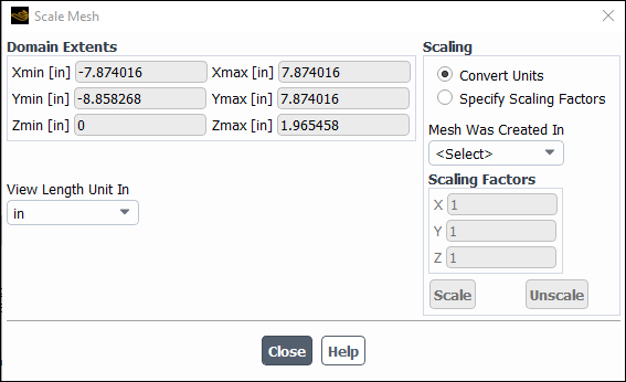
Select in from the View Length Unit In drop-down list to set inches as the working unit for length.
Confirm that the domain extents are as shown in the previous dialog box.
Close the Scale Mesh dialog box.
The working unit for length has now been set to inches.
Note: Because the default SI units will be used for everything except length, there is no need to change any other units in this problem. The choice of inches for the unit of length has been made by the actions you have just taken. If you want a different working unit for length, other than inches (for example, millimeters), click in the Domain ribbon tab (Mesh group box) and make the appropriate change in the Set Units dialog box.
In the steps that follow, you will select a solver and specify physical models, material properties, and zone conditions for your simulation using the Physics ribbon tab.
In the Solver group box of the Physics ribbon tab, retain the default selection of the steady pressure-based solver.
Physics →
Solver → General
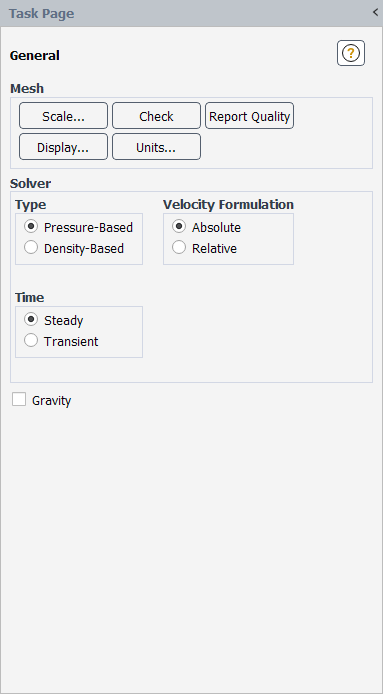
Set up your models for the CFD simulation using the Models group box of the Physics ribbon tab.
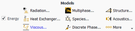
Note: You can also use the Models task page, which can be accessed from the tree by expanding Setup and double-clicking the Models tree item.
Enable heat transfer by activating the energy equation.
In the Physics ribbon tab, enable Energy (Models group box).
Physics → Models
→ Energy
Note: You can also double-click the Setup/Models/Energy tree item and enable the energy equation in the Energy dialog box.
Enable the
 -
- turbulence model. Physics → Models
→ Viscous...
turbulence model. Physics → Models
→ Viscous...
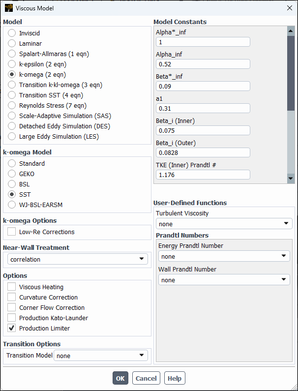
Retain the default selection of k-omega from the Model list.
Retain the default selection of SST in the k-omega Model group box.
Enable the Production Limiter check box in the Options group.
Click to accept all the other default settings and close the Viscous Model dialog box.
Note that the Viscous... label in the ribbon is displayed in blue to indicate that the Viscous model is enabled. Also Energy and Viscous appear as enabled under the Setup/Models tree branch.
Note: While the ribbon is the primary tool for setting up and solving your problem, the tree is a dynamic representation of your case. The models, materials, conditions, and other settings that you have specified in your problem will appear in the tree. Many of the frequently used ribbon items are also available via the right-click functionality of the tree.
Set up the materials for the CFD simulation using the Materials group box of the Physics ribbon tab.
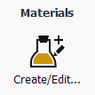
Create a new material called water using the Create/Edit Materials dialog box.
In the Physics ribbon tab, click Create/Edit... (Materials group box).
Physics → Materials
→ Create/Edit...
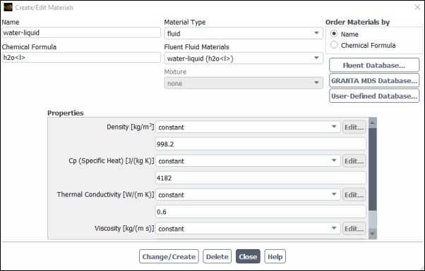
Click the button to access pre-defined materials.
Select water-liquid (h2o < l >) from the Fluent Fluid Materials selection list and click , then close the dialog box.
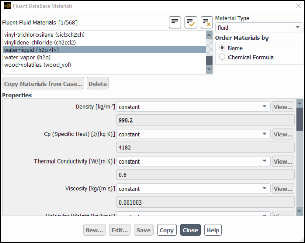
Ensure that there are now two materials (water-liquid and air) defined locally by examining the Fluent Fluid Materials drop-down list.
Both the materials will also be listed under Fluid in the Materials task page and under the Materials tree branch.
Close the Create/Edit Materials dialog box.
Set up the cell zone conditions for the fluid zone (fluid) using the Zones group box of the Physics ribbon tab.
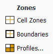
In the Physics tab, click Cell Zones (Zones group box).
Physics → Zones
→ Cell Zones
This opens the Cell Zone Conditions task page.
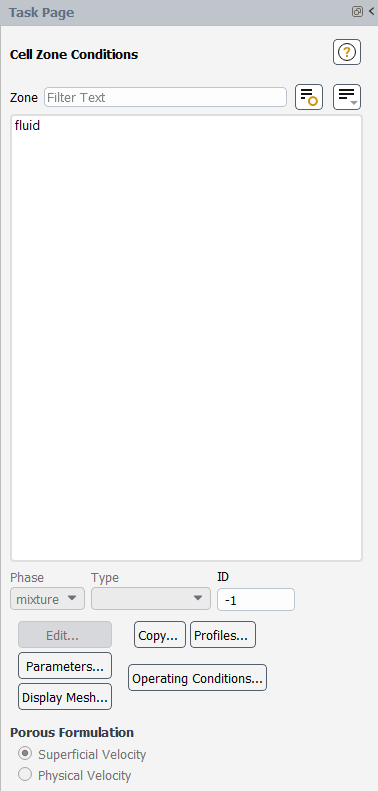
Double-click fluid in the Zone list to open the Fluid dialog box.
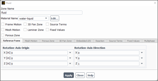
Note: You can also double-click the Setup/Cell Zone Conditions/fluid tree item in order to open the corresponding dialog box.
Select water-liquid from the Material Name drop-down list.
Click and close the Fluid dialog box.
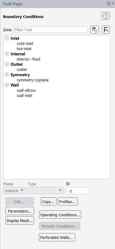
Set up the boundary conditions for the inlets, outlet, and walls for your CFD analysis using the Zones group box of the Physics ribbon tab.
In the Physics tab, click Boundaries (Zones group box).
Physics → Zones
→ Boundaries
This opens the Boundary Conditions task page where the boundaries defined in your simulation are displayed in the Zone selection list.
Note: To display boundary zones grouped by zone type (as shown previously), click the Toggle Tree View button (
 ) in the upper right corner of the Boundary
Conditions task page and select Zone Type under
Group By.
) in the upper right corner of the Boundary
Conditions task page and select Zone Type under
Group By.Here the zones have names that were previously given during the meshing process. It is good practice to give boundaries meaningful names in a meshing application to help when you set up the model. You can also change boundary names in Fluent by simply editing the boundary and making revisions in the Zone Name text box.
Set the boundary conditions at the cold inlet (cold-inlet).
Tip: If you are unsure of which inlet zone corresponds to the cold inlet, you can probe the mesh display using the right mouse button or the probe toolbar button (
 ) as described previously in this tutorial. The information
will be displayed in the Ansys Fluent console, and the zone you probed will be
automatically selected from the Zone selection list in the
Boundary Conditions task page.
) as described previously in this tutorial. The information
will be displayed in the Ansys Fluent console, and the zone you probed will be
automatically selected from the Zone selection list in the
Boundary Conditions task page.Double-click cold-inlet to open the Velocity Inlet dialog box.
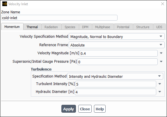
Retain the default selection of Magnitude, Normal to Boundary from the Velocity Specification Method drop-down list.
Enter
0.4[m/s] for Velocity Magnitude.In the Turbulence group box, select Intensity and Hydraulic Diameter from the Specification Method drop-down list.
Retain the default value of
5[%] for Turbulent Intensity.Enter
4[inches] for Hydraulic Diameter.The hydraulic diameter
 is defined as:
where
 is the cross-sectional area and
  is the wetted perimeter.
Click the Thermal tab.
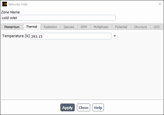
Enter
293.15[K] for Temperature.Click and close the Velocity Inlet dialog box.
Note: You can also access the Velocity Inlet dialog box by double-clicking the Setup/Boundary Conditions/cold-inlet tree item.
In a similar manner, set the boundary conditions at the hot inlet (hot-inlet), using the values in the following table:
Setting Value Velocity Specification Method Magnitude, Normal to Boundary Velocity Magnitude 1.2[m/s]Specification Method Intensity and Hydraulic Diameter Turbulent Intensity 5[%]Hydraulic Diameter 1[inch]Temperature 313.15[K]Double-click outlet in the Boundary Condition selection list and set the boundary conditions at the outlet, as shown in the following figure.
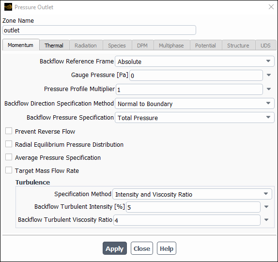
Note:You do not need to set a backflow temperature in this case (in the Thermal tab) because the material properties are not functions of temperature. If they were, a flow-weighted average of the inlet conditions would be a good starting value.
Ansys Fluent will use the backflow conditions only if the fluid is flowing into the computational domain through the outlet. Since backflow might occur at some point during the solution procedure, you should set reasonable backflow conditions to prevent convergence from being adversely affected.
For the wall of the elbow (wall-elbow) and the wall of the hot inlet (wall-inlet), retain the default value of
0W/m2 for Heat Flux in the Thermal tab.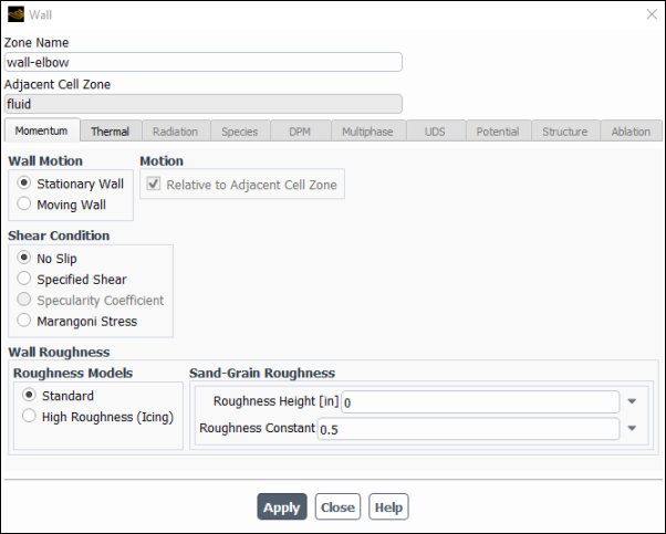

In the steps that follow, you will set up and run the calculation using the Solution ribbon tab.
Note: You can also use the task pages listed under the Solution tree branch to perform solution-related activities.
Select a solver scheme.
In the Solution ribbon tab, click Methods... (Solution group box).
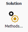 Solution → Solution
→ Methods...
Solution → Solution
→ Methods...
Retain the default settings.
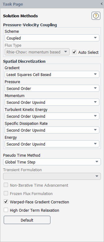
Enable the plotting of residuals during the calculation.
In the Solution ribbon tab, click Residuals... (Reports group box).
 Solution → Reports
→ Residuals...
Solution → Reports
→ Residuals...
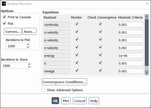
Note: You can also access the Residual Monitors dialog box by double-clicking the Solution/Monitors/Residual tree item.
Ensure that Plot is enabled in the Options group box.
Retain the default value of
0.001for the Absolute Criteria of continuity.Click to close the Residual Monitors dialog box.
Note: By default, the residuals of all of the equations solved for the physical models enabled for your case will be monitored and checked by Ansys Fluent as a means to determine the convergence of the solution. It is a good practice to also create and plot a surface report definition that can help evaluate whether the solution is truly converged. You will do this in the next step.
Create a surface report definition of average temperature at the outlet (outlet).
Solution → Reports
→ Definitions → New
→ Surface Report → Mass-Weighted
Average...
Note: You can also access the Surface Report Definition dialog box by right-clicking Report Definitions in the tree (under Solution) and selecting New/Surface Report/Mass-Weighted Average... from the menu that opens.
Enter
outlet-temp-avgfor the Name of the report definition.Enable Report File, Report Plot, and Print to Console in the Create group box.
During a solution run, Ansys Fluent will write solution convergence data in a report file, plot the solution convergence history in a graphics window, and print the value of the report definition to the console.
Set Frequency to
3by clicking the up-arrow button.This setting instructs Ansys Fluent to update the plot of the surface report, write data to a file, and print data in the console after every 3 iterations during the solution.
Select Temperature... and Static Temperature from the Field Variable drop-down lists.
Select outlet from the Surfaces selection list.
Click to save the surface report definition and close the Surface Report Definition dialog box.
The new surface report definition outlet-temp-avg will appear under the Solution/Report Definitions tree item. Ansys Fluent also automatically creates the following items:
outlet-temp-avg-rfile (under the Solution/Monitors/Report Files tree branch)
outlet-temp-avg-rplot (under the Solution/Monitors/Report Plots tree branch)
Examine the report file settings of the created report definition (outlet-temp-avg-rfile).
 Solution → Monitors
→ Report Files
→ outlet-temp-avg-rfile
Solution → Monitors
→ Report Files
→ outlet-temp-avg-rfile
 Edit...
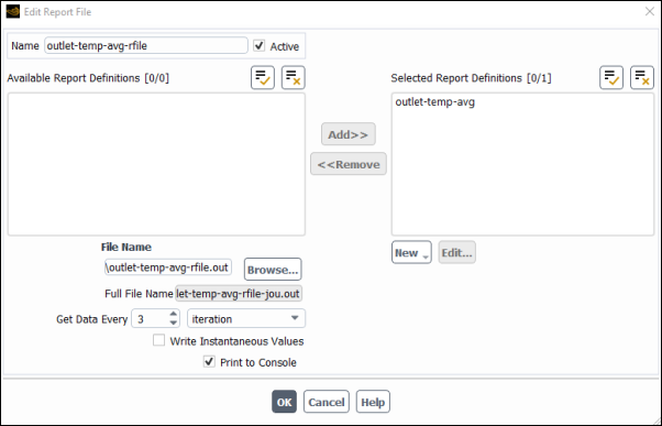
The Edit Report File dialog box is automatically populated with data from the outlet-temp-avg report definition.
Verify that outlet-temp-avg is in the Selected Report Definitions list.
If you had created multiple report definitions, the additional ones would be listed under Available Report Definitions , and you could use the Add>> and <<Remove buttons to manage which were written in this particular report definition file.
(optional) Edit the name and location of the resulting file as necessary using the File Name field or button.
Click to close the Edit Report File dialog box.
Create a convergence condition for outlet-temp-avg.
Solution → Reports
→ Convergence...
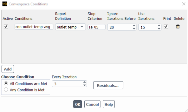
Click the button.
Enter
con-outlet-temp-avgfor Conditions.Select outlet-temp-avg from the Report Definition drop-down list.
Enter
1e-5for Stop Criterion.Enter
20for Ignore Iterations Before.Enter
15for Use Iterations.Enable Print.
Set Every Iteration to
3.Click to save the convergence condition settings and close the Convergence Conditions dialog box.
These settings will cause Fluent to consider the solution converged when the surface report definition value for each of the previous 15 iterations is within 0.001% of the current value. Convergence of the values will be checked every 3 iterations. The first 20 iterations will be ignored, allowing for any initial solution dynamics to settle out. Note that the value printed to the console is the deviation between the current and previous iteration values only.
Initialize the flow field using the Initialization group box of the Solution ribbon tab.
Solution → Initialization
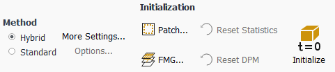
Retain the default selection of Hybrid from the Method list.
Click .
Save the case file (
elbow1.cas.h5). File → Write →
Case...
Start the calculation by requesting 150 iterations in the Solution ribbon tab (Run Calculation group box).
Solution → Run
Calculation
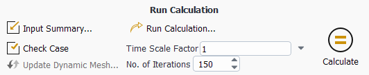
Enter
150for No. of Iterations.Click .
Note: By starting the calculation, you are also starting to save the surface report data at the rate specified in the Surface Report Definition dialog box. If a file already exists in your working directory with the name you specified in the Edit Report File dialog box, then a Question dialog box will open, asking if you would like to append the new data to the existing file. Click in the Question dialog box, and then click in the Warning dialog box that follows to overwrite the existing file.
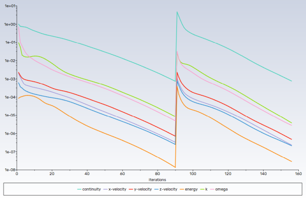
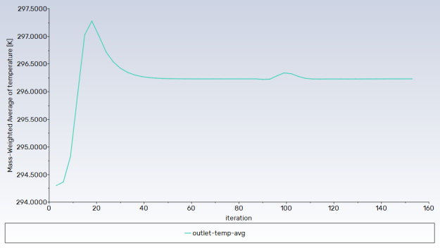
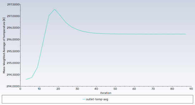
As the calculation progresses, the surface report history will be plotted in the outlet-temp-avg-rplot tab in the graphics window (Figure 5.2: Convergence History of the Mass-Weighted Average Temperature).
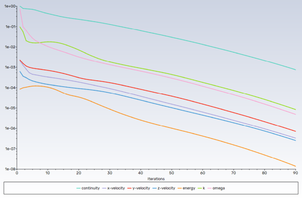
Similarly, the residuals history will be plotted in the Scaled Residuals tab in the graphics window (Figure 5.3: Residuals).
Note: You can monitor the two convergence plots simultaneously by right-clicking a tab in the graphics window and selecting SubWindow View from the menu that opens. To return to a tabbed graphics window view, right-click a graphics window title area and select Tabbed View.
Since the residual values vary slightly by platform, the plot that appears on your screen may not be exactly the same as the one shown here.
The solution will be stopped by Ansys Fluent when any of the following occur:
the surface report definition converges to within the tolerance specified in the Convergence Conditions dialog box
the residual monitors converge to within the tolerances specified in the Residual Monitors dialog box
the number of iterations you requested in the Run Calculation task page has been reached
In this case, the solution is stopped when the convergence criterion on outlet temperature is satisfied. The exact number of iterations for convergence will vary, depending on the platform being used. An Information dialog box will open to alert you that the calculation is complete. Click in the Information dialog box to proceed.
Examine the plots for convergence (Figure 5.2: Convergence History of the Mass-Weighted Average Temperature and Figure 5.3: Residuals).
Note: There are no universal metrics for judging convergence. Residual definitions that are useful for one class of problem are sometimes misleading for other classes of problems. Therefore it is a good idea to judge convergence not only by examining residual levels, but also by monitoring relevant integrated quantities and checking for mass and energy balances.
There are three indicators that convergence has been reached:
The residuals have decreased to a sufficient degree.
The solution has converged when the Convergence Criterion for each variable has been reached. The default criterion is that each residual will be reduced to a value of less than 10–3, except the energy residual, for which the default criterion is 10–6.
The solution no longer changes with more iterations.
Sometimes the residuals may not fall below the convergence criterion set in the case setup. However, monitoring the representative flow variables through iterations may show that the residuals have stagnated and do not change with further iterations. This could also be considered as convergence.
The overall mass, momentum, energy, and scalar balances are obtained.
You can examine the overall mass, momentum, energy and scalar balances in the Flux Reports dialog box. The net imbalance should be less than 0.2 % of the net flux through the domain when the solution has converged. In the next step you will check to see if the mass balance indicates convergence.
Examine the mass flux report for convergence using the Results ribbon tab.
Results → Reports
→ Fluxes...
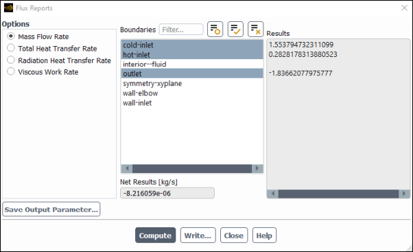
Ensure that Mass Flow Rate is selected from the Options list.
Select cold-inlet, hot-inlet, and outlet from the Boundaries selection list.
Click .
The individual and net results of the computation will be displayed in the Results and Net Results boxes, respectively, in the Flux Reports dialog box, as well as in the console.
The sum of the flux for the inlets should be very close to the sum of the flux for the outlets. The net results show that the imbalance in this case is well below the 0.2% criterion suggested previously.
Close the Flux Reports dialog box.
Save the data file (
elbow1.dat.h5). File → Write →
Data...
In later steps of this tutorial you will save additional case and data files with different suffixes.
In the steps that follow, you will visualize various aspects of the flow for the preliminary solution using the Results ribbon tab.
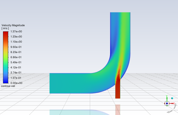
Display filled contours of velocity magnitude on the symmetry plane (Figure 5.4: Predicted Velocity Distribution after the Initial Calculation).
Results → Graphics
→ Contours → New...
Enter
contour-velfor Contour Name.Ensure that Filled is enabled in the Options group box.
Ensure that Node Values and Boundary Values are enabled in the Options group box.
Select Banded in the Coloring group box.
Select Velocity... and Velocity Magnitude from the Contours of drop-down lists.
Select symmetry-xyplane from the Surfaces selection list.
Click to display the contours in the active graphics window. Clicking the blue z-axis arrow in the axis triad will orient the view with the z-axis, and clicking the Fit to Window icon (
 ) will cause the object to fit exactly and be centered in the
window.
) will cause the object to fit exactly and be centered in the
window.Note: If you cannot see the velocity contour display, select the appropriate tab in the graphics window.
Close the Contours dialog box.
Note: When you probe a point in the displayed domain with the right mouse button or the probe tool, the level of the corresponding contour is highlighted in the colormap in the graphics window, and is also reported in the console.
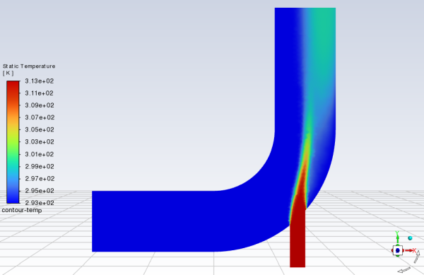
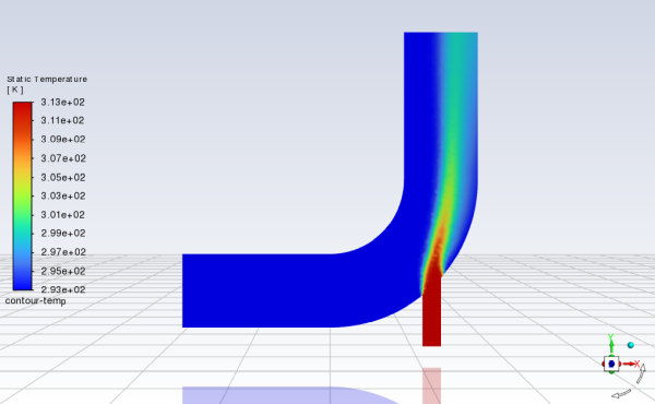
Create and display a definition for temperature contours on the symmetry plane (Figure 5.5: Predicted Temperature Distribution after the Initial Calculation).
Results → Graphics
→ Contours → New...
You can create contour definitions and save them for later use.
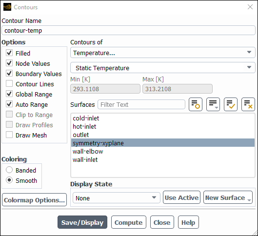
Enter
contour-tempfor Contour Name.Select Temperature... and Static Temperature from the Contours of drop-down lists.
Select symmetry-xyplane from the Surfaces selection list.
Click and close the Contours dialog box.
The new contour-temp definition appears under the Results/Graphics/Contours tree branch. To edit your contour definition, right-click it and select Edit... from the menu that opens.
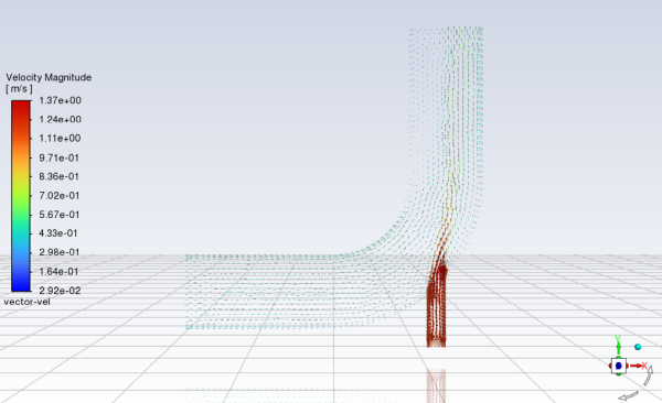
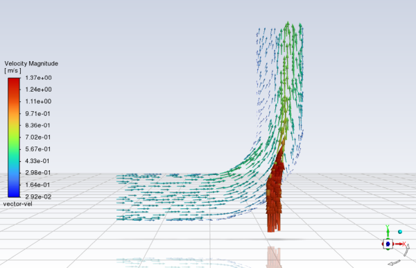
Display velocity vectors on the symmetry plane (Figure 5.8: Magnified View of Resized Velocity Vectors).
Results → Graphics
→ Vectors → New...
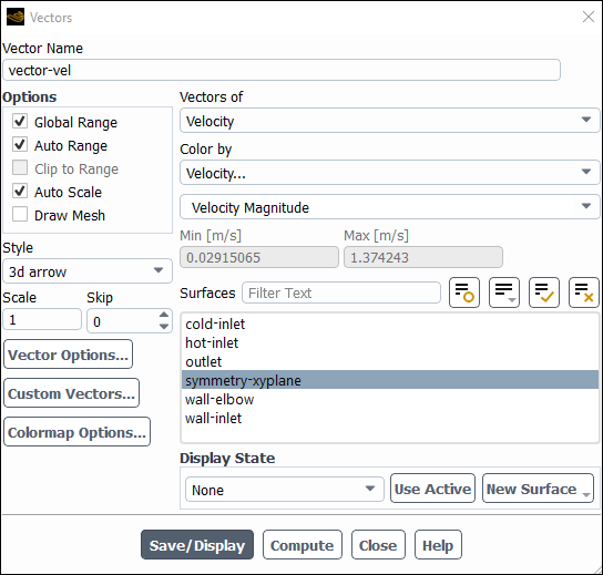
Enter
vector-velfor Vector Name.Select symmetry-xyplane from the Surfaces selection list.
Click to plot the velocity vectors.
The Auto Scale option is enabled by default in the Options group box. This scaling sometimes creates vectors that are too small or too large in the majority of the domain. You can improve the clarity by adjusting the Scale and Skip settings, thereby changing the size and number of the vectors when they are displayed.
Enter
4for Scale.Set Skip to
2.Click again to redisplay the vectors.
Close the Vectors dialog box.
Zoom in on the vectors in the display.
Zoom out to the original view.
Clicking the Fit to Window icon,
 , will cause the object to fit exactly and be centered in the
window.
, will cause the object to fit exactly and be centered in the
window.
Create a line at the centerline of the outlet. For this task, you will use the Surface group box of the Results tab.
 Results → Surface
→ Create → Iso-Surface...
Results → Surface
→ Create → Iso-Surface...
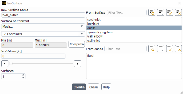
Enter
z=0_outletfor New Surface Name.Select Mesh... and Z-Coordinate from the Surface of Constant drop-down lists.
Click to obtain the extent of the mesh in the z-direction.
The range of values in the z-direction is displayed in the Min and Max fields.
Retain the default value of
0inches for Iso-Values.Select
outletfrom the From Surface selection list.Click .
The new line surface representing the intersection of the plane z=0 and the surface
outletis created, and its name z=0_outlet appears in the From Surface selection list.
Note:After the line surface z=0_outlet is created, a new entry will automatically be generated for New Surface Name, in case you would like to create another surface.
If you want to delete or otherwise manipulate any surfaces, click Manage... to open the Surfaces dialog box.
Close the Iso-Surface dialog box.
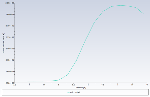
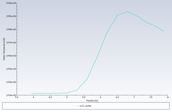
Display and save an XY plot of the temperature profile across the centerline of the outlet for the initial solution (Figure 5.9: Outlet Temperature Profile for the Initial Solution).
Results → Plots
→ XY Plot → New...
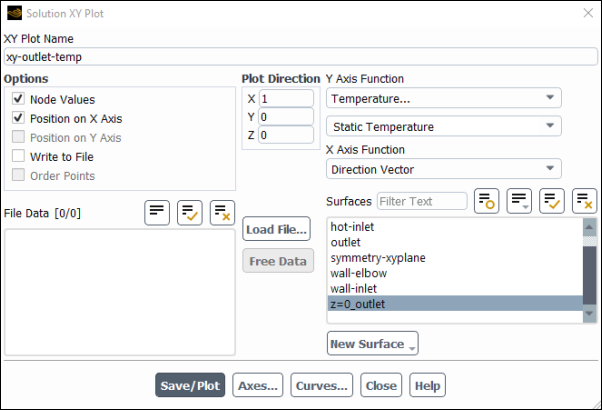
Enter
xy-outlet-tempfor XY Plot Name.Select Temperature... and Static Temperature from the Y Axis Function drop-down lists.
Select the z=0_outlet surface you just created from the Surfaces selection list.
Click .
Enable Write to File in the Options group box.
The button that was originally labeled will change to .
Click .
In the Select File dialog box, enter
outlet_temp1.xyfor XY File.Click to save the temperature data and close the Select File dialog box.
Close the Solution XY Plot dialog box.
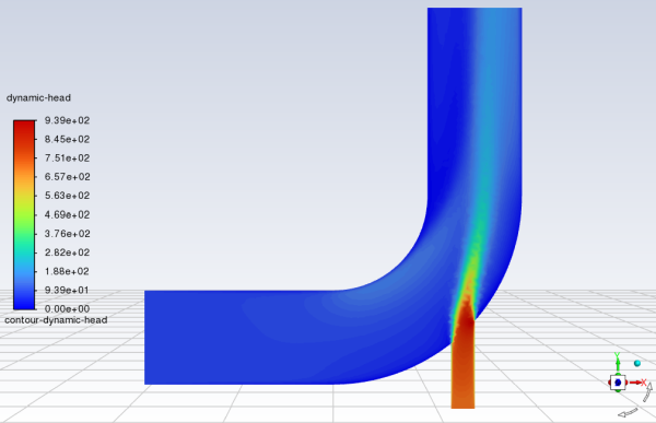
Define a custom field function for the dynamic head formula (
 ). User Defined → Field
Functions → Custom...
). User Defined → Field
Functions → Custom...
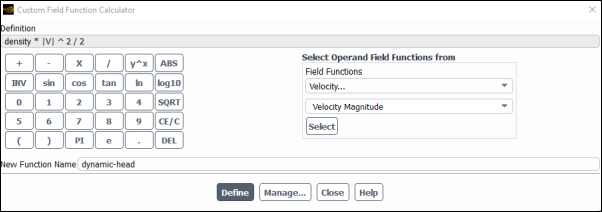
Select Density... and Density from the Field Functions drop-down lists, and click the button to add density to the Definition field.
Click the button to add the multiplication symbol to the Definition field.
Select Velocity... and Velocity Magnitude from the Field Functions drop-down lists, and click the button to add |V| to the Definition field.
Click to raise the last entry in the Definition field to a power, and click for the power.
Click the button to add the division symbol to the Definition field, and then click .
Enter
dynamic-headfor New Function Name.Click and close the Custom Field Function Calculator dialog box.
The dynamic-head tree item will appear under the Parameters & Customization/Custom Field Functions tree branch.
Display filled contours of the custom field function (Figure 5.10: Contours of the Dynamic Head Custom Field Function).
Results → Graphics
→ Contours → New...
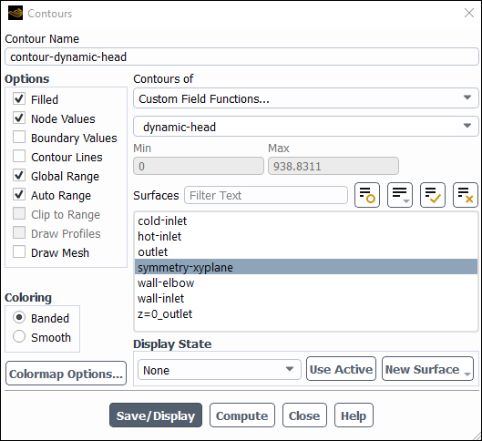
Enter
contour-dynamic-headfor Contour Name.Select Banded in the Coloring group box.
Disable Boundary Values in the Options group.
Select Custom Field Functions... and dynamic-head from the Contours of drop-down lists.
Tip: Custom Field Functions... is at the top of the upper Contours of drop-down list.
Select symmetry-xyplane from the Surfaces selection list.
Click and close the Contours dialog box.
Note: You may need to change the view by zooming out after the last vector display, if you have not already done so.
Save the settings for the custom field function by writing the case and data files (
elbow1.cas.h5andelbow1.dat.h5). File → Write →
Case & Data...
Ensure that
elbow1.cas.h5is entered for Case/Data File.Note: When you write the case and data file at the same time, it does not matter whether you specify the file name with a
.casor.datextension, as both will be saved.Click to save the files and close the Select File dialog box.
Click to overwrite the files that you had saved earlier.

For the first run of this tutorial, you have solved the elbow problem using a fairly coarse mesh. The elbow solution can be improved further by refining the mesh to better resolve the flow details. Ansys Fluent provides a built-in capability to easily adapt (locally refine) the mesh according to solution gradients. In the following steps you will adapt the mesh based on the temperature gradients in the current solution and compare the results with the previous results.
Define Cell Registers to adapt the mesh in the regions of high temperature gradient.
Solution → Cell
Registers New →
Field Variable...
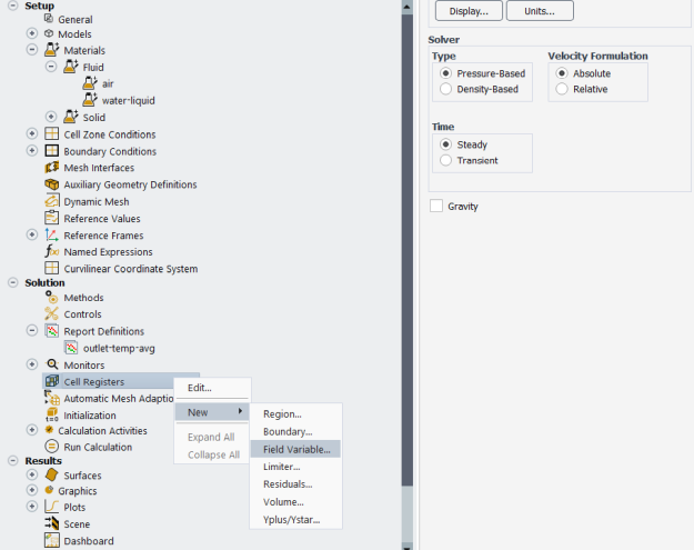
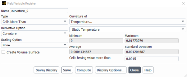
Select Cells More Than from the Type drop-down list.
Select Curvature from the Derivative Option drop-down list.
Select Temperature... and Static Temperature from the Curvature of drop-down list.
Click .
Ansys Fluent will update the Minimum and Maximum values to show the minimum and maximum temperature gradient. The Average temperature gradient and Standard Deviation will also be displayed.
Enter a value of
0.0015for the Cells having value more than.A general rule is to use about 10% of the maximum gradient when setting the value for refinement.
Click and close the Field Variable Register dialog box.
Set up mesh adaption using the Cell Registers. For this task, you will use the Adapt group box in the Domain ribbon tab.
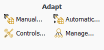 Domain → Adapt
→ Manual...
Domain → Adapt
→ Manual...
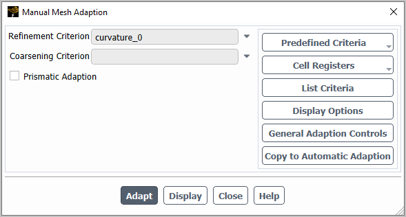
Select the previously defined curvature_0 cell register from the Refinement Criterion drop-down lists.
Ansys Fluent will not coarsen beyond the original mesh for a 3D mesh. Hence, it is not necessary to select the Coarsening Criterion in this instance.
Click .
Click .
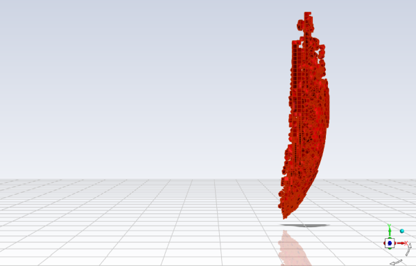
Ansys Fluent will display the cells marked for adaption in the graphics window (Figure 5.11: Cells Marked for Adaption).
Extra — You can change the way Ansys Fluent displays cells marked for adaption (Figure 5.12: Alternative Display of Cells Marked for Adaption) by performing the following steps:
Click in the Manual Mesh Adaption dialog box to open the Display Options - Adaption dialog box.
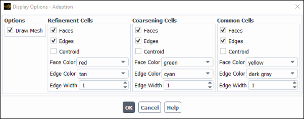
Enable Draw Mesh in the Options group box.
The Mesh Display dialog box will open.
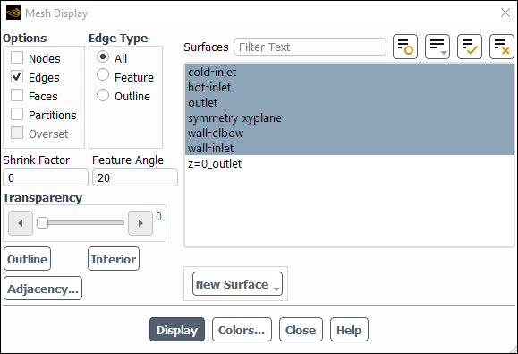
Ensure that only the Edges option is enabled in the Options group box.
Select All from the Edge Type list.
Select all of the items except z=0_outlet from the Surfaces selection list.
Click and close the Mesh Display dialog box.
Click to close the Display Options - Adaption dialog box.
Click in the Manual Mesh Adaption dialog box.
Rotate the view and zoom in to get the display shown in Figure 5.12: Alternative Display of Cells Marked for Adaption.
After viewing the marked cells, rotate the view back and zoom out again.
Click to close the Manual Mesh Adaption dialog box.
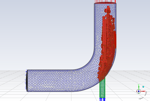
Display the adapted mesh (Figure 5.13: The Adapted Mesh).
Domain → Mesh
→ Display...
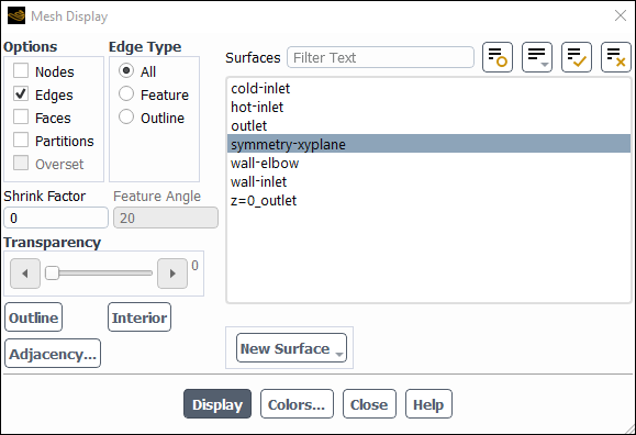
Disable Faces in the Options group box.
Select All from the Edge Type list.
Deselect all of the highlighted items from the Surfaces selection list except for symmetry-xyplane.
Tip: To deselect all surfaces, click the button (
 ) at the top of the Surfaces selection
list. Then select the desired surface from the Surfaces
selection list.
) at the top of the Surfaces selection
list. Then select the desired surface from the Surfaces
selection list.Click and close the Mesh Display dialog box.
Request an additional 150 iterations.
Solution → Run
Calculation → Calculate
The solution will converge as shown in Figure 5.14: The Complete Residual History and Figure 5.15: Convergence History of Mass-Weighted Average Temperature.
Save the case and data files for the solution with an adapted mesh (
elbow2.cas.h5andelbow2.dat.h5). File → Write →
Case & Data...
Enter
elbow2.cas.h5for Case/Data File.Click to save the files and close the Select File dialog box.
The files
elbow2.cas.h5andelbow2.dat.h5will be saved in your default folder.Display the temperature distribution (using node values) on the revised mesh using the temperature contours definition that you created earlier (Figure 5.16: Filled Contours of Temperature Using the Adapted Mesh).
Right-click the Results/Graphics/Contours/contour-temp tree item and select Display from the menu that opens.
Results → Graphics
→ Contours → contour-temp
Display
Display and save an XY plot of the temperature profile across the centerline of the outlet for the adapted solution (Figure 5.17: Outlet Temperature Profile for the Adapted Coupled Solver Solution).
Results → Plots
→ XY Plot → xy-outlet-temp
Edit...
Click Save/Plot to display the XY plot.
Enable Write to File in the Options group box.
The button that was originally labeled Save/Plot will change to Write....
Click .
In the Select File dialog box, enter
outlet_temp2.xyfor XY File.Click to save the temperature data.
Close the Solution XY Plot dialog box.
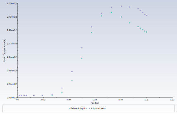
Display the outlet temperature profiles for both solutions on a single plot (Figure 5.18: Outlet Temperature Profiles for the Two Solutions).
Open the Plot Data Sources dialog box.
Results → Plots
→ Data Sources...
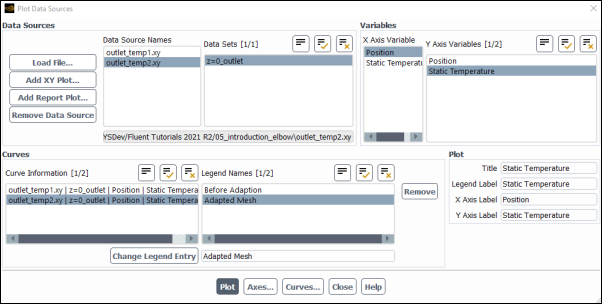
Click the button to open the Select File dialog box.
Select outlet_temp1.xy and outlet_temp2.xy.
Each of these files will be listed with their folder path in the bottom list to indicate that they have been selected.
Tip: If you select a file by mistake, simply click the file in the bottom list and then click .
Click to save the files and close the Select File dialog box.
Select the folder path ending in outlet_temp1.xy from the Curve Information selection list (Curves group box).
Enter
Before Adaptionin the lower-right text-entry box.Click the button.
The item in the Legend Entries list for outlet_temp1.xy will be changed to Before Adaption. This legend entry will be displayed in the upper-left corner of the XY plot generated in a later step.
In a similar manner, change the legend entry for the folder path ending in outlet_temp2.xy to be
Adapted Mesh.Click and close the Plot Data Sources dialog box.
Figure 5.18: Outlet Temperature Profiles for the Two Solutions shows the two temperature profiles at the centerline of the outlet. It is apparent by comparing both the shape of the profiles and the predicted outer wall temperature that the solution is highly dependent on the mesh and solution options. Specifically, further mesh adaption should be used in order to obtain a solution that is independent of the mesh.