Chapter 4: Modeling External Compressible Flow

This tutorial is divided into the following sections:

4.1. Introduction

Note: This tutorial is fully supported at all licensing levels.

The purpose of this tutorial is to compute the turbulent flow past a transonic wing at a nonzero angle of attack. You will use the k-ω SST turbulence model.

This tutorial demonstrates how to do the following:

Creation of capsule mesh using Watertight Geometry workflow.
Model compressible flow (using the ideal gas law for density).
Set boundary conditions for external aerodynamics.
Use the k-ω SST turbulence model.
Calculate a solution using the pressure-based coupled solver with global time step selected for the pseudo time method.
Check the near-wall mesh resolution by plotting the distribution of .

Related video that demonstrates steps for setting up, solving, and postprocessing the solution results for a turbulent flow within a manifold:

4.2. Prerequisites

This tutorial is written with the assumption that you have completed the introductory tutorials found in this manual and that you are familiar with the Ansys Fluent outline view and ribbon structure. Some steps in the setup and solution procedure will not be shown explicitly.

4.3. Problem Description

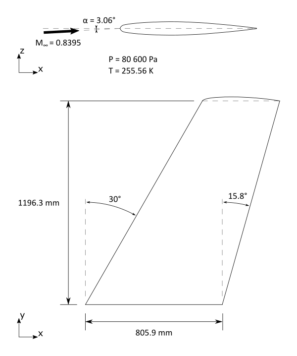
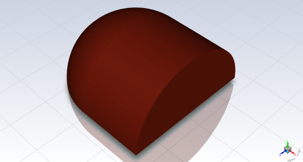
The problem considers the flow around a wing at an angle of attack α=3.06° and a free stream Mach number of 0.8395 (M_∞=0.8395). The flow is transonic, and has a shock near the mid-chord (x/c≃0.20) on the upper (suction) side. The wing has a mean aerodynamic chord length of 0.64607 m, a span of 1.1963 m, an aspect ratio of 3.8, and a taper ratio of 0.562. The geometry of the wing is shown in Figure 4.1: Problem Specification.

Figure 4.1: Problem Specification

4.4. Setup and Solution

The following sections describe the setup and solution steps for this tutorial:

4.4.1. Preparation

To prepare for running this tutorial:

Download the external_compressible.zip file here .
Unzip external_compressible.zip to your working directory.
The SpaceClaim CAD file wing.scdoc can be found in the folder.
Use the Fluent Launcher to start Ansys Fluent.
Select Meshing in the top-left selection list to start Fluent in Meshing Mode.
Enable Double Precision under Options.
Set Meshing Processes and Solver Processes to 4 under Parallel (Local Machine).

4.4.2. Meshing Workflow

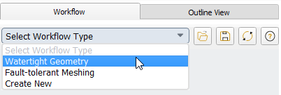
Start the meshing workflow.
1. In the Workflow tab, select the Watertight Geometry workflow.
2. Review the tasks of the workflow.
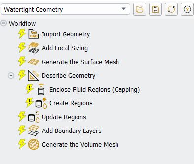
  Each task is designated with an icon indicating its state (for example, as complete, incomplete, etc. For more information, see Understanding Task States in the Fluent User's Guide). All tasks are initially incomplete and you proceed through the workflow completing all tasks. Additional tasks are also available for the workflow. For more information, see Customizing Workflows in the Fluent User's Guide.
Import the CAD geometry (wing.scdoc).
1. Select the Import Geometry task.
2. For Units, keep the default setting as mm.
3. For File Name, enter the path and file name for the CAD geometry that you want to import (wing.scdoc).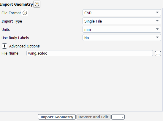
  Note: The workflow only supports *.scdoc (SpaceClaim), Workbench (.agdb), and the intermediary *.pmdb file formats.
4. Click Import Geometry.
  This will update the task, display the geometry in the graphics window (Figure 3.2: The Imported CAD Geometry for the Catalytic Converter), and allow you to proceed onto the next task in the workflow.
  Figure 4.2: The Imported CAD Geometry for the Wing
  
  The wing geometry has been encased in a half-spherical, half-cylindrical volume with 25m of space in all directions.
  Note: Alternatively, you can use the ... button next to File Name to locate the CAD geometry file, after which, the Import Geometry task automatically updates, displaying the geometry in the graphics window, and the workflow automatically progresses to the next task.
  Throughout the workflow, you are able to return to a task and change its settings using either the Edit button, or the Revert and Edit button.
Add local sizing.
1. In the Add Local Sizing task, you are prompted as to whether or not you would like to add local sizing controls to the faceted geometry.
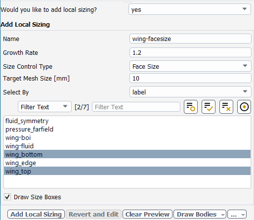
  In this tutorial, we will add local sizing around the wing and a region past the trailing edge, since they are areas where we require a more refined mesh. Later, we will apply settings for a coarser surface mesh elsewhere.
  1. At the prompt for adding local sizing, select yes.
  2. Enter wing-facesize for the Name of the size control.
  3. Retain Face Size for the Size Control Type.
  4. Specify 10 for the Target Mesh Size.
  5. Select wing_bottom and wing_top.
2. Click Add Local Sizing task, you are prompted as to whether or not you would like to add local sizing controls to the faceted geometry.
  You can now see the wing task in the workflow, which can be selected to change its settings. The Add Local Sizing task can still be used to add more local sizing controls to the geometry.
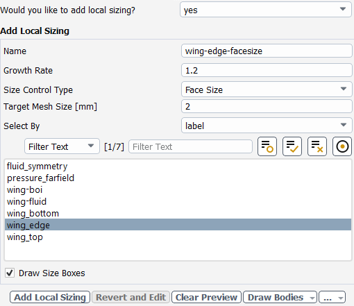
  1. At the prompt for adding local sizing, select yes.
  2. Enter wing-edge-facesize for the Name of the size control.
  3. Retain Face Size for the Size Control Type.
  4. Specify 2 for the Target Mesh Size.
  5. Select wing_edge.
3. Click Add Local Sizing.
  You can now see the wing task in the workflow, which can be selected to change its settings. The Add Local Sizing task can still be used to add more local sizing controls to the geometry.
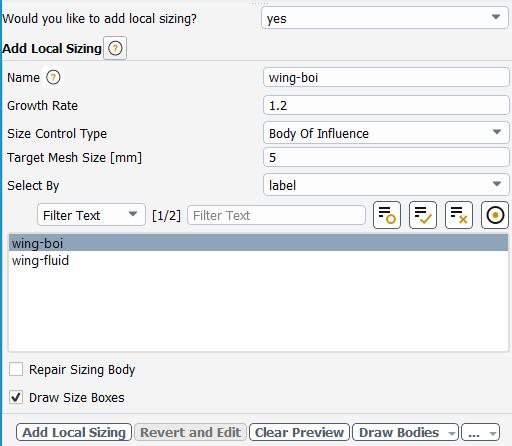
  1. Select Body Of Influence for the Size Control Type.
  2. Enter wing-boi for the Name of the size control.
  3. Specify 5 for the Target Mesh Size.
  4. Select wing-boi.
  5. Click Add Local Sizing to complete this task and proceed to the next task in the workflow.
Generate the surface mesh.
1. In the Generate the Surface Mesh task, you can set various properties of the surface mesh for the faceted geometry.
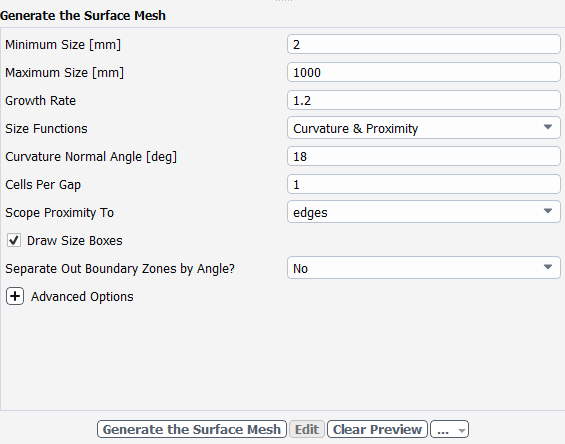
2. Specify 2 for the Minimum Size.
3. Specify 1000 for the Maximum Size.
  Note: The red boxes displayed on the geometry in the graphics window are a graphical representation of size settings. These boxes change size as the values change, and they can be hidden by using the Clear Preview button.
4. Click Generate the Surface Mesh to complete this task and proceed to the next task in the workflow.
Describe the geometry.
When you select the Describe Geometry task, you are prompted with questions relating to the nature of the imported geometry.
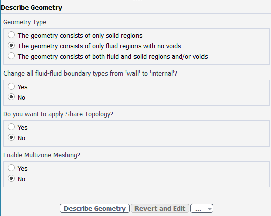
1. Select The geometry consists of only fluid regions with no voids option under Geometry Type, since this model contains only the fluid region.
2. Keep the rest of the default settings for this task.
3. Click Describe Geometry to complete this task and proceed to the next task in the workflow.
Confirm and update the boundaries.
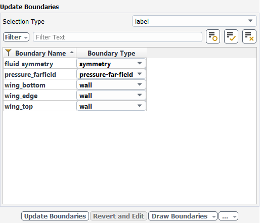
1. Select the Update Boundaries task, where you can inspect the mesh boundaries and confirm and change any designated boundaries accordingly. Ansys Fluent attempts to determine the correct arrangement of boundaries automatically.
2. All the proposed boundaries are correct, so click Update Boundaries. and proceed to the next task.
Update your regions.
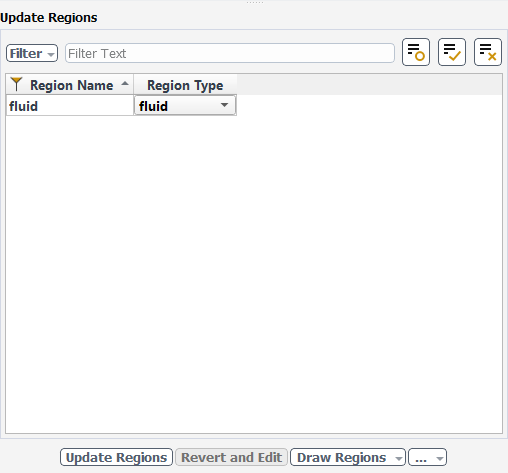
1. Select the Update Regions task, where you can review and change the tabulated names and types of the various regions that have been generated from your imported geometry, and change them as needed.
  We can see that the only defined region is the fluid region.
2. The proposed region type is correct, so click Update Regions to update your settings.
Add boundary layers.
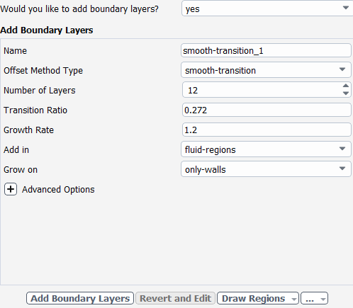
1. Select the Add Boundary Layers task, where you can set properties of the boundary layer mesh.
  For the Add Boundary Layers task, ensure yes is selected at the prompt as to whether or not you want to define boundary layer settings. In this task, you can define specific details for capturing the boundary layer in and around your geometry.
2. Specify 12 for Number of Layers.
  Many boundary layers are desired to model a well resolved flow near the wall.
3. Click Add Boundary Layers.
Generating the volume mesh.
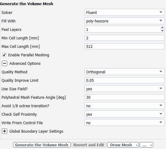
1. Select the Generate the Volume Mesh task, where you can set properties of the volume mesh itself.
2. Select the poly-hexcore for Fill With.
3. Specify 512 for Max Cell Length.
4. Enable Advanced Options to expose additional options that are required for this task.
  Select yes for Check Self Proximity.
5. Click Generate the Volume Mesh.
  Ansys Fluent will apply your settings and proceed to generate a volume mesh for the wing geometry.. The mesh is displayed in the graphics window and a clipping plane is automatically inserted with a layer of cells drawn so that you can quickly see the details of the volume mesh.
Check the mesh.
Mesh → Check → Perform Mesh Check
Save the mesh file (wing.msh.h5).
File → Write → Mesh...
Switch to Solution mode.
Now that a mesh has been generated using Ansys Fluent in meshing mode, you can now switch to solver mode to complete the set up of the simulation. Note that to obtain more accurate solutions a higher quality mesh should be used.
We have just checked the mesh, so select Yes when prompted to switch to solution mode.

4.4.3. Mesh

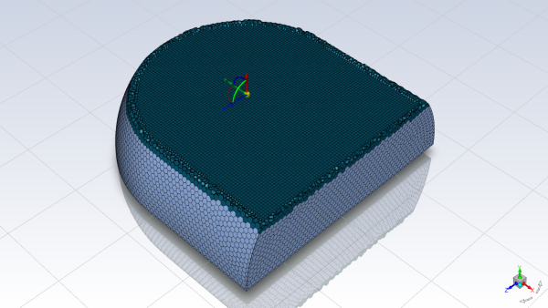
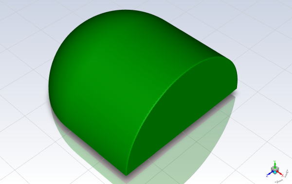
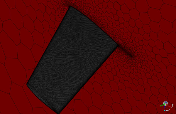
Examine the mesh (Figure 4.3: The Entire Mesh and Figure 4.4: Magnified View of the Mesh Around the Wing).
Figure 4.3: The Entire Mesh

To examine the cells of the mesh around the wing, display the mesh with edges enabled and the far-field boundary disabled.
Domain → Mesh → Display...
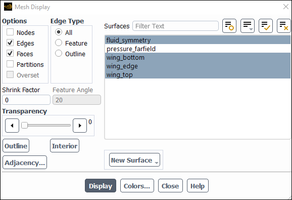
1. Enable Edges in the Options group box.
2. Ensure All is selected in the Edge Type group box.
3. Deselect pressure-farfield from the Surfaces selection list.
4. Click Display and close the Mesh Display dialog box.
5. Zoom in on the region around the wing, as shown in Figure 4.4: Magnified View of the Mesh Around the Wing.
Figure 4.4: Magnified View of the Mesh Around the Wing

The cells near the surface have a relatively higher resolution and high aspect ratios, to account for the flow around the wing.
Note: You can use the right mouse button to probe for mesh information in the graphics window. If you click the right mouse button on any node in the mesh, information will be displayed in the Ansys Fluent console about the associated zone, including the name of the zone. This feature is especially useful when you have several zones of the same type and you want to distinguish between them quickly.

4.4.4. Solver

Set the solver settings.
Setup → General
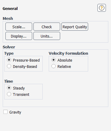
1. Retain the default selection of Pressure-Based from the Type list.
  The pressure-based solver with the Coupled option for the pressure-velocity coupling is a good alternative to density-based solvers of Ansys Fluent when dealing with applications involving high-speed aerodynamics with shocks. Selection of the coupled algorithm is made in the Solution Methods task page in the Solution step.

4.4.5. Models

Select the k-ω SST turbulence model.
Physics → Models → Viscous...
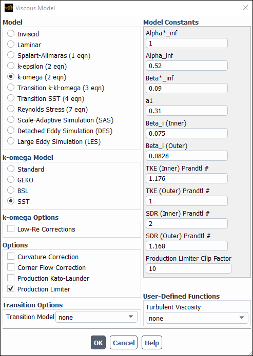
1. Retain the default selection of k-omega (2 eqn) in the Model list.
2. Retain the default selection of SST in the k-omega Model list.
3. Click OK to close the Viscous Model dialog box.

4.4.6. Materials

The default Fluid Material is air, which is the working fluid in this problem. The default settings need to be modified to account for compressibility and variations of the thermophysical properties with temperature.

Set the properties for air, the default fluid material.
Setup → Materials → Fluid → air Edit...
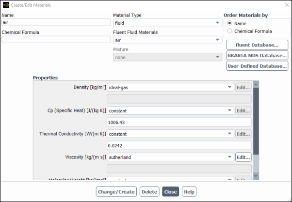
1. Select ideal-gas from the Density drop-down list.
  The Energy Equation will be enabled.
2. Select sutherland from the Viscosity drop-down list to open the Sutherland Law dialog box.
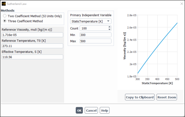
  1. Retain the default selection of Three Coefficient Method in the Methods list.
  2. Click OK to close the Sutherland Law dialog box.
  The Sutherland law for viscosity is well suited for high-speed compressible flows.
3. Click Change/Create to save these settings.
4. Close the Create/Edit Materials dialog box.
While Density and Viscosity have been made temperature-dependent, Cp (Specific Heat) and Thermal Conductivity have been left constant. For high-speed compressible flows, thermal dependency of the physical properties is generally recommended. For simplicity, Thermal Conductivity and Cp (Specific Heat) are assumed to be constant in this tutorial.

4.4.7. Boundary Conditions

Setup → Boundary Conditions

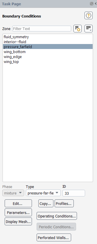
Set the boundary conditions for pressure_farfield.
Setup → Boundary Conditions → pressure_farfield → Edit...
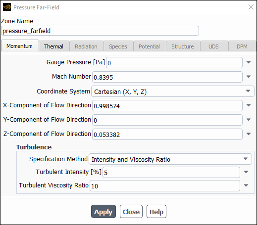
1. Retain the default value of 0 Pa for Gauge Pressure.
  Note: The gauge pressure in Ansys Fluent is always relative to the operating pressure, which is defined in a separate input (see below).
2. Enter 0.8395 for Mach Number.
3. Enter 0.998574 and 0.053382 for the X-Component of Flow Direction and Z-Component of Flow Direction, respectively.
  These values are determined by the 3.06° angle of attack: cos 3.06°≃0.998574 and sin 3.06°≃0.053382
4. Retain Intensity and Viscosity Ratio from the Specification Method drop-down list in the Turbulence group box.
5. Retain the default value of 5% for Turbulent Intensity and 10 for Turbulent Viscosity Ratio.
  The viscosity ratio should be between 1 and 10 for external flows.
6. Click the Thermal tab and enter 255.56 K for Temperature.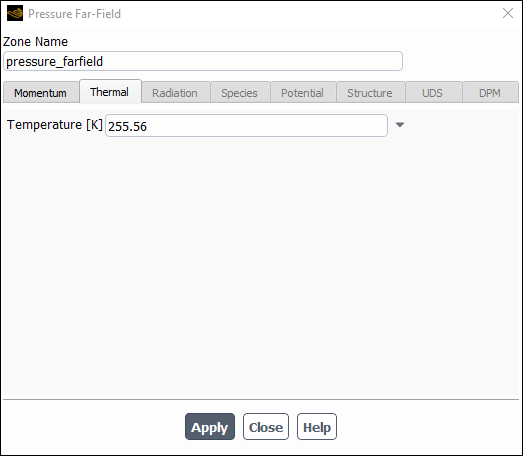
7. Click Apply and close the Pressure Far-Field dialog box.

4.4.8. Operating Conditions

Set the operating pressure.
Setup → Boundary Conditions → Operating Conditions...

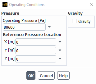
The Operating Conditions dialog box can also be accessed from the Cell Zone Conditions task page.
1. Enter 80600 Pa for Operating Pressure.
  The operating pressure should be set to a meaningful mean value in order to avoid round-off errors. The absolute pressure must be greater than zero for compressible flows. If you want to specify boundary conditions in terms of absolute pressure, you can make the operating pressure zero.
2. Click OK to close the Operating Conditions dialog box.

For information about setting the operating pressure, see the Fluent User's Guide.

4.4.9. Reference Values

Set the reference values that are used to compute the pressure coefficient.
Setup → Reference Values
The reference values are used to non-dimensionalize physical quantities used for postprocessing. The dimensionless pressure coefficient will be used in future steps.
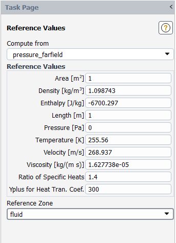
1. Select pressure_farfield from the Compute from drop-down list.
  Ansys Fluent will update the Reference Values based on the boundary conditions at the far-field boundary.

4.4.10. Solution

Set the solution parameters.
Solution → Solution → Methods...

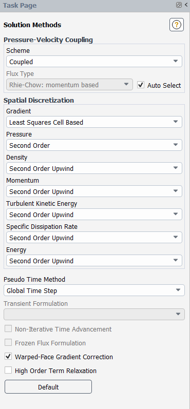
Retain the default settings.
Enable residual plotting during the calculation.
Solution → Reports → Residuals...
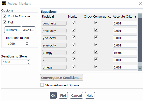
1. Ensure that Plot is enabled in the Options group box and click OK to close the Residual Monitors dialog box.
Initialize the solution.
Solution → Initialization
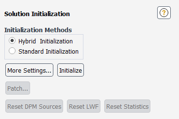
1. Retain the default selection of Hybrid Initialization from the Initialization Methods group box.
2. Click Initialize to initialize the solution.
Save the case files (wing.cas.h5).
File → Write → Case...
Start the calculation by requesting 150 iterations.
Solution → Run Calculation → Run Calculation...
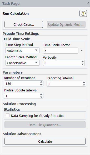
1. Enter 5 for the Time Scale Factor.
  The Time Scale Factor allows you to further manipulate the computed time step size calculated by Ansys Fluent. Larger time steps can lead to faster convergence. However, if the time step is too large it can lead to solution instability.
2. Enter 150 for Number of Iterations.
3. Click Calculate.
Save the case and data files (wing.cas.h5 and wing.dat.h5).
File → Write → Case & Data...

4.4.11. Postprocessing

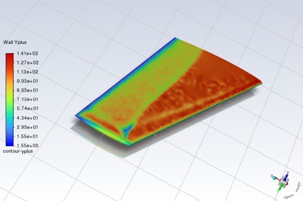
Plot the distribution on the wing (Figure 4.5: Contour Plot of y+ Distribution).
Results → Graphics → Contours → New...
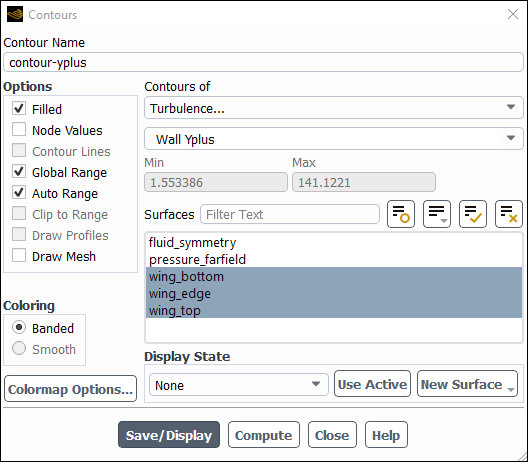
1. Enter contour-yplus for Contour Name.
2. Disable Node Values in the Options group box.
3. Select Turbulence... and Wall Yplus from the Contours of drop-down lists.
4. Select wing_bottom, wing_edge, and wing_top from the Surfaces selection list.
5. Click Save/Display and close the Contours dialog box.
Note: The values of are dependent on the resolution of the mesh and the Reynolds number of the flow, and are defined only in wall-adjacent cells. The value of in the wall-adjacent cells dictates how wall shear stress is calculated.
The equation for is
(4–1)
where is the distance from the wall to the cell center, is the molecular viscosity, is the density of the air, and is the wall shear stress.
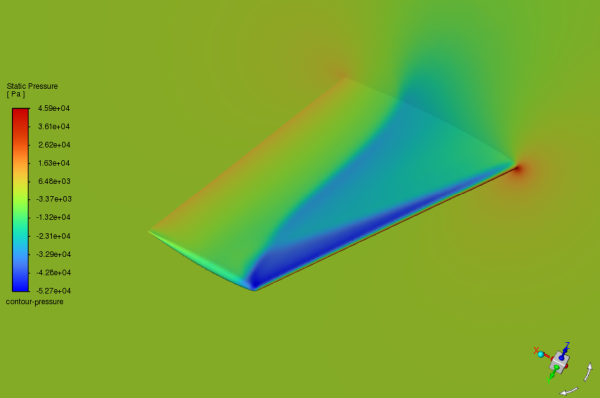
For this tutorial, the relatively coarse mesh was prepared with a target max value of ~100, as indicated in Figure 4.5: Contour Plot of y+ Distribution.
Figure 4.5: Contour Plot of y+ Distribution
Plot the pressure distribution on the wing (Figure 4.6: Contour Plot of Pressure).
Results → Graphics → Contours → New...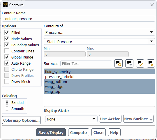
1. Enter contour-pressure for Contour Name.
2. Enable Banded in the Coloring group box.
3. Select Pressure... and Static Pressure from the Contours of drop-down lists.
4. Select fluid_symmetry, wing_bottom, wing_edge, and wing_top from the Surfaces selection list.
5. Click Save/Display.
  Figure 4.6: Contour Plot of Pressure
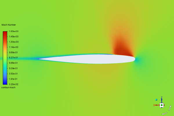
Create a plane near the shock region.
Results → Surface → Create → Plane...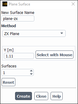
1. Enter plane-zx for New Surface Name.
2. Select ZX Plane from the Method drop-down lists.
3. Enter 1.11 m for Y.
  This value corresponds to the y-coordinate at around the shock region near the tip of the wing. Alternatively, you can click Select with Mouse to select a point from the graphics window.
4. Click Create and close the Plane Surface dialog box.
Plot the Mach number distribution on the wing near the shock region (Figure 4.7: Contour Plot of Mach Number).
Results → Graphics → Contours → New...
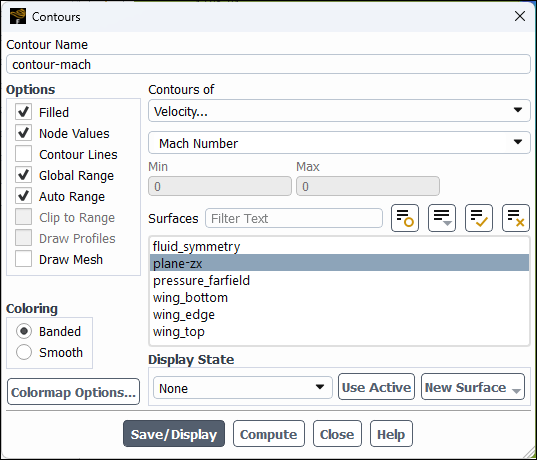
1. Enter contour-mach for Contour Name.
2. Enable Banded in the Coloring group box.
3. Select Velocity... and Mach Number from the Contours of drop-down list.
4. Select plane-zx from the From Surface selection list.
5. Click Save/Display and close the Contours dialog box.
6. Zoom in on the region around the wing, as shown in Figure 4.7: Contour Plot of Mach Number.
  Figure 4.7: Contour Plot of Mach Number
  
  Note the discontinuity, in this case a shock, on the upper surface of the wing in Figure 4.7: Contour Plot of Mach Number at about x/c≃0.20.
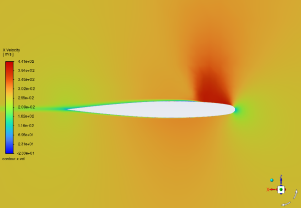
Display filled contours of the component of velocity (Figure 4.8: Contour Plot of x Component of Velocity).
Results → Graphics → Contours → New...
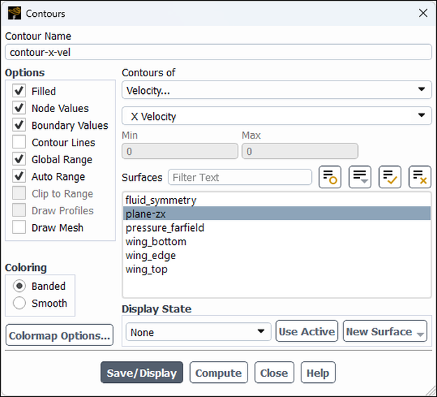
1. Enter contour-x-vel for Contour Name.
2. Ensure Filled is enabled in the Options group box.
3. Enable Banded in the Coloring group box.
4. Select Velocity... and X Velocity from the Contours of drop-down lists.
5. Select plane-zx from the From Surface selection list.
6. Click Save/Display and close the Contours dialog box.
Note the flow reversal downstream of the shock in Figure 4.8: Contour Plot of x Component of Velocity.
Figure 4.8: Contour Plot of x Component of Velocity
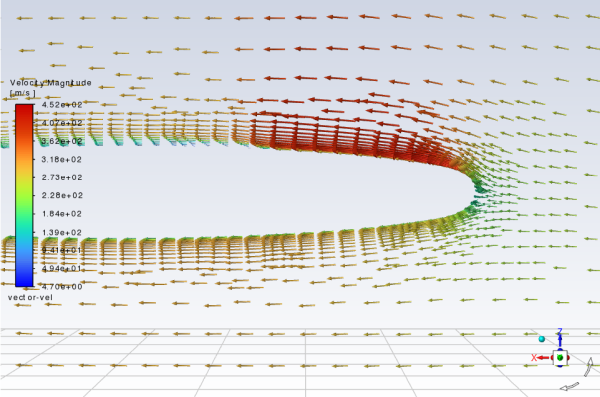
Plot velocity vectors (Figure 4.9: Plot of Velocity Vectors Downstream of the Shock).
Results → Graphics → Vectors → New...
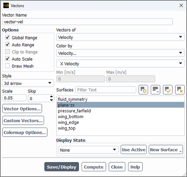
1. Enter vector-vel for Vector Name.
2. Enter 0.05 for Scale.
3. Select Velocity... and X Velocity from the Color by drop-down lists.
4. Select plane-zx from the From Surface selection list.
5. Click Save/Display and close the Vectors dialog box.
6. Zoom in on the flow above the upper surface at a point downstream of the shock, as shown in Figure 4.9: Plot of Velocity Vectors Downstream of the Shock.
Figure 4.9: Plot of Velocity Vectors Downstream of the Shock

Flow reversal is clearly visible in Figure 4.9: Plot of Velocity Vectors Downstream of the Shock.
Create iso-surfaces near the shock region.
Results → Surface → Create → Iso-Surface...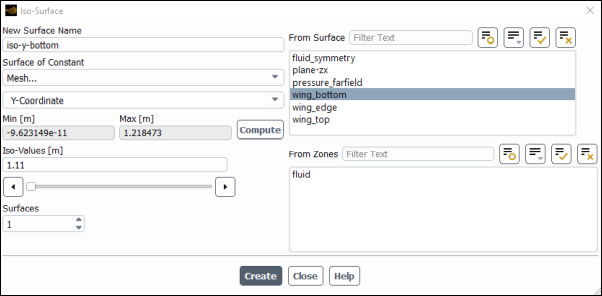
1. Enter iso-y-bottom for New Surface Name.
2. Select Mesh... and Y-Coordinate from the Surface of Constant drop-down lists.
3. Select wing_bottom from the From Surface selection list.
4. Click Compute and enter 1.11 m for Iso-Values.
  This value corresponds to the y-coordinate at the shock region near the tip of the wing.
5. Click Create.
6. Similarly, create a surface iso-y-top from the wing_top surface.
7. Close the Iso-Surface dialog box.
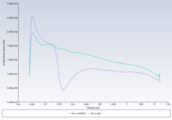
Plot the component of wall shear stress on the wing near the shock region (Figure 4.10: XY Plot of x Wall Shear Stress).
Results → Plots → XY Plot → New...
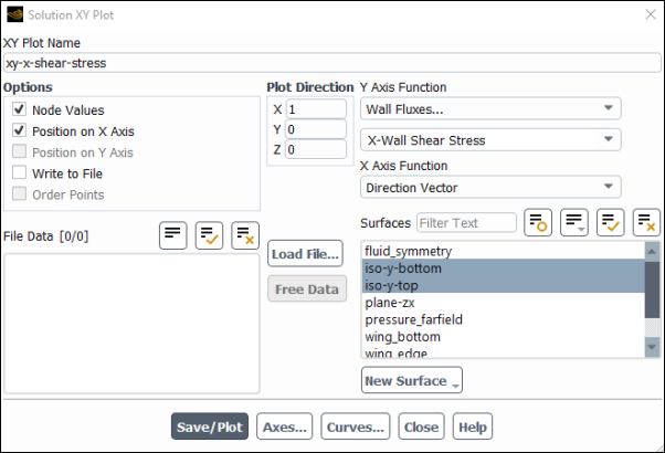
1. Enter xy-x-shear-stress for XY Plot Name.
2. Select Wall Fluxes... and X-Wall Shear Stress from the Y Axis Function drop-down lists.
3. Select iso-y-bottom and iso-y-top from the Surfaces selection list.
4. Click Save/Plot and close the Solution XY Plot dialog box.
As shown in Figure 4.10: XY Plot of x Wall Shear Stress, the large, adverse pressure gradient induced by the shock causes the boundary layer to separate. The point of separation is where the wall shear stress vanishes. Flow reversal is indicated here by negative values of the x component of the wall shear stress.
Figure 4.10: XY Plot of x Wall Shear Stress
Save the case file (wing.cas.h5).
File → Write → Case...

4.5. Summary

This tutorial demonstrated how to set up and solve an external aerodynamics problem using poly-hexcore meshing, the pressure-based coupled solver with under-relaxation from a pseudo time method and the k-ω SST turbulence model.