Chapter 32: Simulating a 1P3S Battery Pack Using the Battery Model

This tutorial is divided into the following sections:

32.1. Introduction

This tutorial is used to show how to set up a battery pack (battery system connected in parallel/series pattern) simulation in Ansys Fluent. All the three submodels are available for a pack simulation.

This tutorial illustrates how to do the following:

Set up a battery pack simulation using the NTGK battery submodel in Ansys Fluent
Define active, tab, and busbar conductive zones
Define electric contacts for the contact surface and external connectors
Define electric conductivity for the active material using the user-defined scalars
Define electric conductivity for the passive material using the user-defined function
Obtain the battery pack simulation results and perform postprocessing activities

Most problem setup procedures are similar to the single cell simulation. The differences in the problem setup will be emphasized in this tutorial.

32.2. Prerequisites

This tutorial is written with the assumption that you have completed the introductory tutorials found in this manual and that you are familiar with the Ansys Fluent outline view and ribbon structure. Some steps in the setup and solution procedure will not be shown explicitly.

32.3. Problem Description

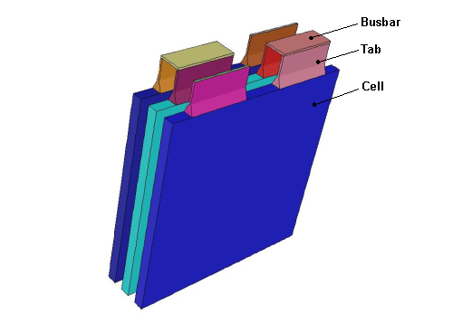
This problem considers a small 1P3S battery pack, that is, the three battery cells connected in series. A schematic of the problem is shown in Figure 32.1: Schematic of the Battery Pack Problem.

Figure 32.1: Schematic of the Battery Pack Problem

The discharging process of the battery pack is occurring under constant power of 200 W. The nominal cell capacity is 14.6 Ah.

You will create a material for the battery cells (an active material) and define the electric conductivity for the active material using the user-defined scalars (UDS). You will create a material for busbars and tabs (a passive material) and define the electric conductivity for the passive material using the provided user-defined function (UDF). You will use the same material for busbars and tabs.

In this tutorial, you will use the NTGK battery submodel to simulate the discharging process under constant power conditions.

32.4. Setup and Solution

The following sections describe the setup and solution steps for this tutorial:

32.4.1. Preparation

Download the battery_pack.zip file here .
Unzip battery_pack.zip to your working directory.
The mesh file 1P3S_battery_pack.msh.h5 can be found in the folder.
Use the Fluent Launcher to start Ansys Fluent.
Select Solution in the top-left selection list to start Fluent in Solution Mode.
Select 3D under Dimension.
Enable Double Precision under Options.
Set Solver Processes to 1 under Parallel (Local Machine).

32.4.2. Reading and Scaling the Mesh

Read the mesh file 1P3S_battery_pack.msh.h5.
File → Read → Mesh...
When prompted, browse to the location of the 1P3S_battery_pack.msh.h5 and select the file.
Once you read in the mesh, it is displayed in the embedded graphics windows.
Check the mesh.
Domain → Mesh → Check → Perform Mesh Check
Scale the mesh.
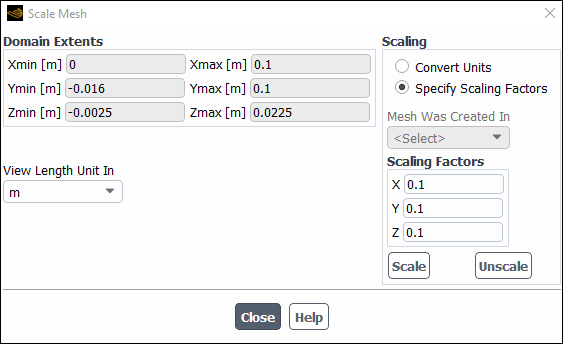
Domain → Mesh → Scale
1. In the Scale Mesh dialog box, select Specify Scaling Factors in the Scaling group.
2. Enter 0.1 for X, Y and Z in the Scaling Factors group.
3. Click Scale and close the Scale Mesh dialog box.
4. Right click in the graphics window and select Refresh Display.
5. Click the Fit to Window icon, , to fit and center the mesh in the graphics window.
Check the mesh.
Domain → Mesh → Perform Mesh Check

32.4.3. Battery Model Setup

The following sections describe the setup steps for this tutorial:

32.4.3.1. Specifying Solver and Models

Enable a time-dependent calculation by selecting Transient in the General task page (Solver group).
Setup → General → Transient

Enable the battery model.

Physics → Models → More → Battery Model

In the Battery Model dialog box, select Enable Battery Model.
The dialog box expands to display the battery model’s settings.
Figure 32.2: Model Options

Once you enable the battery model, the Energy equation will be automatically enabled in order to solve for the temperature field.
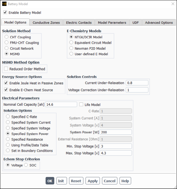
Under the Model Options tab (Figure 32.2: Model Options), configure the following battery operation conditions:
1. Under E-Chemistry Models, enable NTGK/DCIR Empirical Model.
2. In the Electrical Parameters group, retain the default value of 14.6 Ah for Nominal Cell Capacity.
3. Select Enable Joule heat in passive zones in the Energy Source Options group.
4. Enable Specified System Power in the Solution Options group and set System Power to 200 W.
Under the Model Parameters tab, retain the default settings for Y and U coefficients.

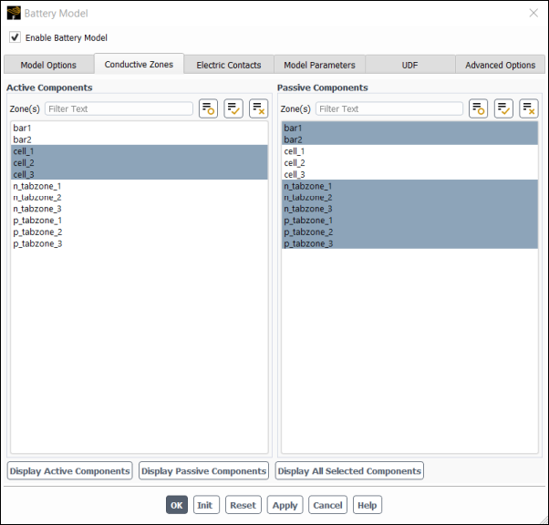
Under the Conductive Zones tab (Figure 32.3: Conductive Zones), configure the following settings:

Group	Control or List	Value or Selection
Active Components	Zone (s)	cell_1
		cell_2
		cell_3
Passive Components	Zone (s)	n_tabzone_1
		n_tabzone_2
		n_tabzone_3
		p_tabzone_1
		p_tabzone_2
		p_tabzone_3
		bar1
		bar2

Figure 32.3: Conductive Zones

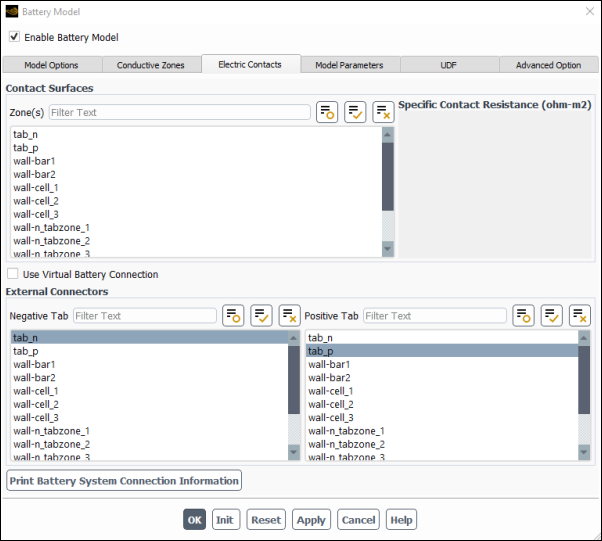
Under the Electric Contacts tab (Figure 32.4: Electric Contacts), configure the contact surface and external connector settings as follows:

Group	Control or List	Value or Selection
External Connectors	Negative Tab	tab_n
External Connectors	Positive Tab	tab_p

The corresponding current or voltage boundary condition will be applied to those boundaries automatically.

Figure 32.4: Electric Contacts

Click the Print Battery System Connection Information button.

Ansys Fluent prints the battery connection information in the console window:

Battery Network Zone Information:
-------------------------------------
 Battery 1s1p
      Active zone:  cell_1
 Battery 2s1p
      Active zone:  cell_2
 Battery 3s1p
      Active zone:  cell_3

 Passive zone 0:
        n_tabzone_1
 Passive zone 1:
        p_tabzone_1
        bar1
        n_tabzone_2
 Passive zone 2:
        p_tabzone_2
        bar2
        n_tabzone_3
 Passive zone 3:
        p_tabzone_3
-------------------------------------

Number of battery series stages =3;  Number of batteries in parallel per series stage=1
****************END OF BATTERY CONNECTION INFO**************

Verify that the connection information is correct. If an error message appears or if the connections are not what you want, redefine the conductive zones in the Conductive Zones tab (Figure 32.3: Conductive Zones). Repeat this process until you confirm that the battery connections are set correctly.
Important: To set a valid connection, you must connect the negative tab to the positive tab through conductive zones.
Click OK to close the Battery Model dialog box.
In the background, Fluent automatically hooks all the necessary UDFs for the problem.
Click OK to close the Information dialog box.

32.4.3.2. Defining New Materials

Define the new e_material material for all the battery’s cells and busbar_material material for the battery pack’s busbars and tabs.

Create the electric material.
Setup → Materials → Solid → aluminum Edit...
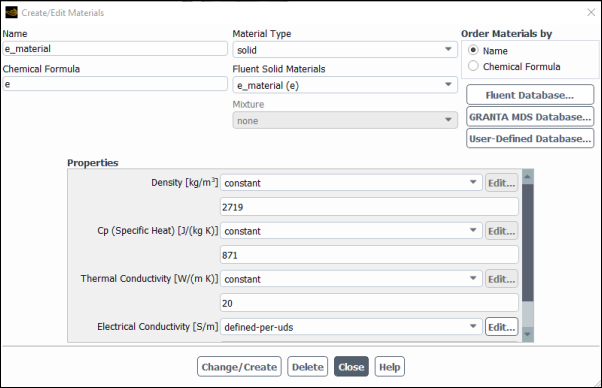
1. In the Create/Edit Materials dialog box, enter e_material for Name and e for Chemical Formula.
2. Set Thermal Conductivity to 20.
3. Under Properties, ensure that defined-per-uds is selected from the Electrical Conductivity drop-down list and click Edit... next to Electrical Conductivity.
4. In the UDS Diffusion Coefficients dialog box, set the constant value of 1.0 e6 for the both user-defined scalars.
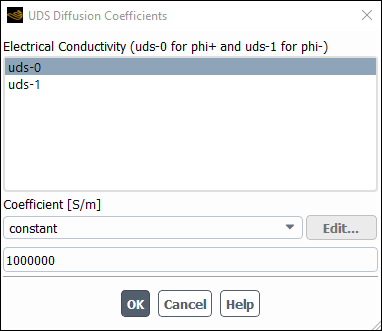
  1. Select uds-0 in the User-Defined Scalar Diffusion list.
  2. Retain constant from the Coefficient drop-down list.
  3. Set 1.0 e6 [1/ohm-m] for Coefficient.
  4. In a similar way, set uds-1 to 1.0 e6 [1/ohm-m] and click OK to close the UDS Diffusion Coefficients dialog box.
5. In the Question dialog box, click No to retain aluminum and add the new material (e_material) to the materials list.
6. Ensure that e_material (e) is selected from the Fluent Solid Materials drop-down list.
7. Close the Create/Edit Material dialog box.
Create the busbar_material material for busbars and tabs by modifying e-material you have created in the previous step.
Setup → Materials → Solid → e-material Edit...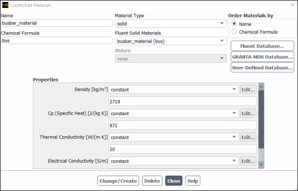
As stated in the problem description, you will use the same material for busbars and tabs.
Note: If the busbar and tab materials are different, you need to define the two different materials and assign them to the busbars and tabs, respectively.
1. In the Create/Edit Materials dialog box, enter busbar_material for Name and bus for Chemical Formula.
2. Set Thermal Conductivity to 20.
3. Enter a value of 3.541 e7 [1/ohm-m] for Electrical Conductivity.
4. Click Change/Create.
5. In the Question dialog box, click No to retain e_material and add the new material (busbar_material) to the materials list.
6. Ensure that busbar_material (bus) is selected from the Fluent Solid Materials drop-down list.
7. Close the Create/Edit Materials dialog box.

32.4.3.3. Defining Cell Zone Conditions

Assign e_material to all the cell zones and busbar_material to all the tabs and busbars.

Assign e_material to the cell_1 cell zone.
Setup → Cell Zone Conditions → cell_1 → Edit...
1. In the Solid dialog box, select e_material from the Material Name drop-down list.
2. Click Apply and close the Solid dialog box.
Copy the cell zone condition for the cell_1 zone to the cell_2 and cell_3 cell zones.
Setup → Cell Zone Conditions → cell_1 → Copy...
1. In the Copy Conditions dialog box, select cell_1 in the From Cell Zone list.
2. In the To Cell Zones list, select cell_2 and cell_3.
3. Click Copy.
4. Click OK in the Question dialog box to copy the cell zone conditions and close the Copy Conditions dialog box.
In a similar manner, assign busbar_material to all the tabs and busbars cell zones.

32.4.3.4. Defining Boundary Conditions

Define the thermal boundary conditions for all walls for the cells, busbars, and tabs. The boundary conditions for the two UDSs have been set automatically when you defined the cell zone conditions.

Set the convection boundary condition for wall-cell_1.
Physics → Zones → Boundaries
1. In the Boundary Conditions task page, select wall-cell_1 and click Edit....
2. In the Wall dialog box, under the Thermal tab, configure the following settings:
  1. Under Thermal Conditions, enable Convection.
  2. Set Heat Transfer Coefficient to 5 [w/m²K].
  3. Set Free Stream Temperature to 300 [K].
  4. Click Apply and close the Wall dialog box.
Copy the boundary conditions for wall-cell_1 to wall-cell_2, wall-cell_3 and all the tab and busbar wall zones (all boundary zones that have names starting with the "wall" string and containing the "bar" or "tabzone" string).
Setup → Boundary Conditions → wall-cell_1 → Copy...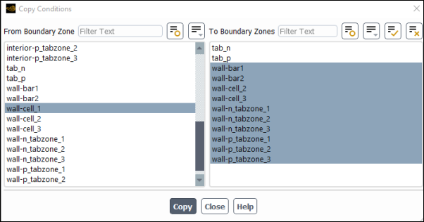

32.4.3.5. Specifying Solution Settings

Turn off the flow and turbulence equations.
Solution → Controls → Equations...
1. In the Equations dialog box, deselect Flow and Turbulence from the Equation selection list.
2. Click OK.
Remove the convergence criteria to ensure that automatic convergence checking does not occur.
Solution → Reports → Residuals...
1. In the Residual Monitors dialog box, enable Show Advanced Options.
2. Select none from the Convergence Criterion drop-down list.
3. Click OK.
Create a surface report definition for the voltage at the positive tab.
Solution → Reports → Definitions → New → Surface Report → Area-Weighted Average...
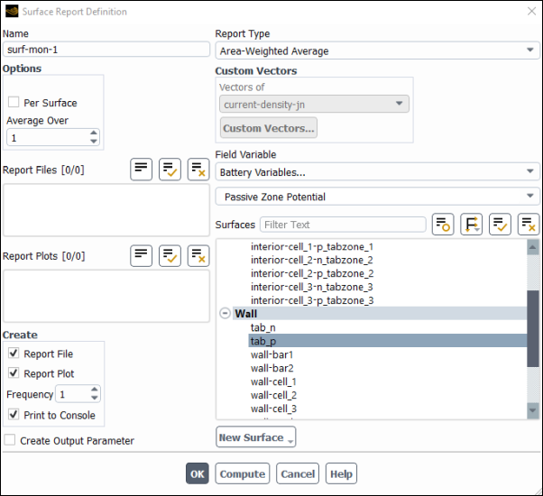
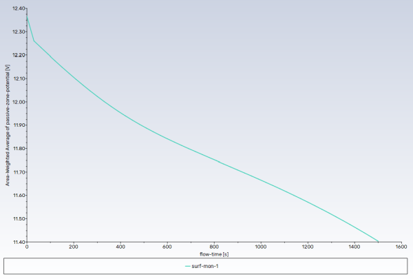
1. In the Surface Report Definition dialog box, enter surf-mon-1 for Name.
2. Select Battery Variables... and Passive Zone Potential from the Field Variable drop-down lists.
3. From the Surfaces selection list, select tab_p.
4. In the Create group box, enable Report Plot and Print to Console.
5. Click OK to save the surface report definition and close the Surface Report Definition dialog box.
6. Modify the attributes of the plot axes.
  Solution → Monitors → Report Plots → surf-mon-1-rplot Edit...
  1. In the Edit Report Plot dialog box, under the Plot Window group box, click the Axes... button to open the Axes dialog box.
  2. Select the X axis and set Precision to 0.
  3. Click Apply.
  4. Select the Y axis and set Precision to 2.
  5. Click Apply and close the Axes dialog box.
    Note: You must click Apply to save the modified settings for each axis.
  6. Ensure that time-step is selected from the Get Data Every drop-down list.
  7. Click OK to close the Edit Report Plot dialog box.
Create a volume report definition to monitor the maximum temperature in the domain.
Solution → Reports → Definitions → New → Volume Report → Max...
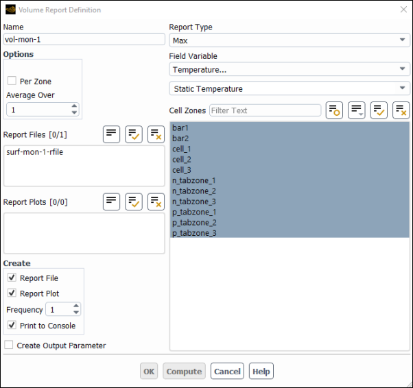
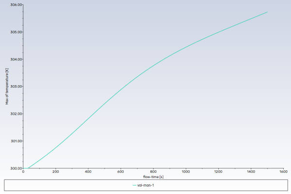
1. In the Volume Report Definition dialog box, enter vol-mon-1 for Name.
2. Select Temperature... and Static Temperature from the Field Variable drop-down lists.
3. From the Cell Zones selection list, select all zones.
4. In the Create group box, enable Report Plot and Print to Console.
5. Click OK to save the volume report definition settings and close the Volume Report Definition dialog box.
6. Modify the attributes of the plot axes.
  Solution → Monitors → Report Plots → vol-mon-1-rplot Edit...
  1. In the Edit Report Plot dialog box, under the Plot Window group box, click the Axes... button to open the Axes dialog box.
  2. Select the X axis and set Precision to 0.
  3. Click Apply.
  4. Select the Y axis and set Precision to 2.
  5. Click Apply and close the Axes dialog box.
  6. Ensure that time-step is selected from the Get Data Every drop-down list.
  7. Click OK to close the Edit Report Plot dialog box.
Save the case file (1P3S_battery_pack.cas.h5).
File → Write → Case...

32.4.3.6. Obtaining Solution

Initialize the field variables using the Standard Initialization method.
Solution → Initialization
1. Retain the selection of Standard from the Initialization Methods group box.
2. Click Initialize.
  Note: Warning messages are printed in the Fluent console informing you about interior zones between different solids. Such messages appear when two adjacent solid zones separated by an interior face type are using two different materials. The message suggests using the mesh/modify-zones/slit-interior-between-diff-solids text command to slit the interior zone between solid zones of differing materials to create a wall/wall-shadow interfaces. In general, the material property interpolation at wall/wall-shadow is more accurate if different materials are used at two sides of an interface. However, the battery model is implemented in such a way that both treatments are equivalent, and such messages could be ignored..
  You do not need to modify the Initial Values in the Solution Initialization task page, because these values are not used for initialization. The Ansys Fluent solver automatically computes the initial condition for UDS0 and UDS1.
Run the simulation.
Solution → Run Calculation
1. Set Time Step Size to 30 seconds and No. of Time Steps to 50.
2. Click Calculate and run the simulation up to 1500 seconds.
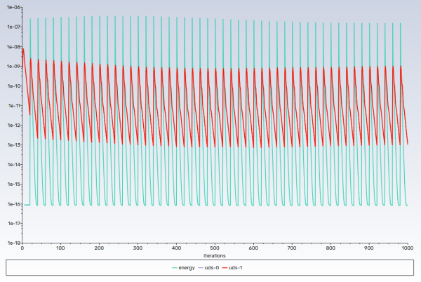
  The residual plot, the history of the voltage at the positive tab and the history of the maximum temperature in the domain are shown in Figure 32.5: Residual History of the Simulation, Figure 32.6: Surface Report Plot of Discharge Curve at 200W, and Figure 32.7: Volume Report Plot of Maximum Temperature in the Domain, respectively.
  Figure 32.5: Residual History of the Simulation
  
  Figure 32.6: Surface Report Plot of Discharge Curve at 200W
  
  Figure 32.7: Volume Report Plot of Maximum Temperature in the Domain
3. Save the case and data files (1P3S_battery_pack.cas.h5 and 1P3S_battery_pack.dat.h5).
  File → Write → Case & Data...

32.4.4. Postprocessing

In this section, postprocessing options for the MSMD battery model solution are presented.

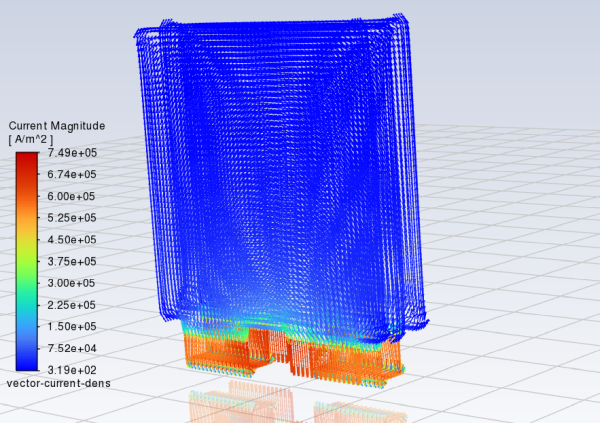
Display the vector plot of current density.
Results → Graphics → Vectors → New...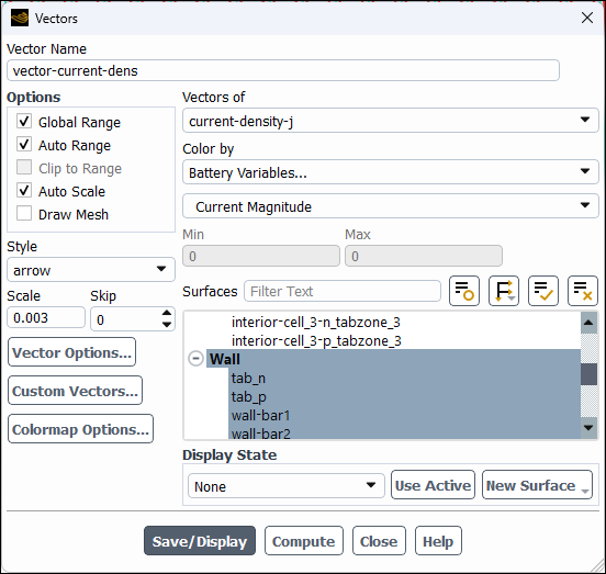
1. Enter vector-current-dens for Vector Name
2. In the Vectors dialog box, select current-density-j from the Vectors of drop-down list.
3. Select Battery Variables... and Current Magnitude from the Color by drop-down list.
4. Click the Toggle Tree View button next to the Surfaces filter and from the drop-down list, select Surface Type (under Group By).
5. From the Surfaces selection list, select Wall.
  The surfaces of the "wall" type are automatically selected in the Surfaces list.
6. In the Options group, enable Draw Mesh and set the mesh display options as desired.
7. Select arrow from the Style drop-down list.
8. Set Scale to 0.003.
9. Click Vector Options....
  1. In the Vector Options dialog box, enable Fixed Length.
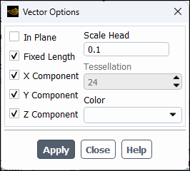
    All vectors in your plot will be displayed with the same lengths.
  2. Set Scale Head to 0.1.
  3. Click Apply and close the Vector Options dialog box.
10. Click Save/Display and close the Vectors dialog box.
  Figure 32.8: Vector Plot of Current Density
  
  Note: Use the Headlight and Lighting display options under the View ribbon tab to manipulate the graphics display.
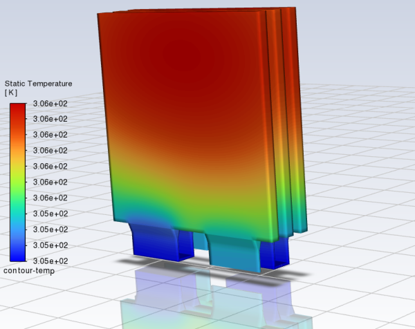
Display the contour plot of the temperature.
Results → Graphics → Contours → New...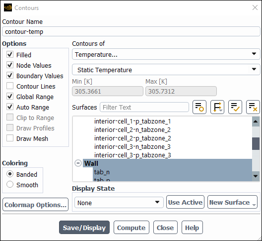
1. Enter contour-temp for Contour Name.
2. Select Banded in the Coloring group box.
3. From the Contours of drop-down list, select Temperature... and Static Temperature.
4. Click the Toggle Tree View button next to the Surfaces filter and from the drop-down list, select Surface Type (under Group By).
5. From the Surfaces selection list, select Wall.
6. Click Save/Display and close the Contours dialog box.
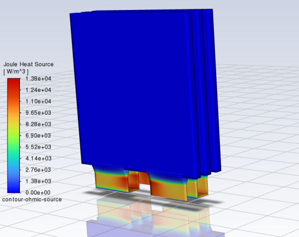
  Figure 32.9: Contour Plot of Temperature
In a similar manner, display the contour of Ohmic heat source.
Results → Graphics → Contours → New...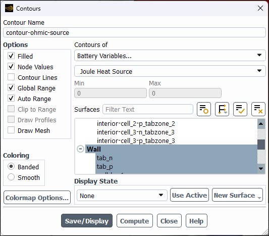
1. Enter contour-ohmic-source for Contour Name.
2. Select Banded in the Coloring group box.
3. From the Contours of drop-down list, select Battery Variables... and Joule Heat Source.
4. From the Surfaces selection list, select Wall.
5. Click Save/Display and close the Contours dialog box.
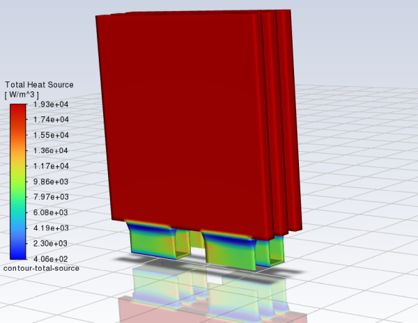
Figure 32.10: Ohmic Heat Generation Rate
In a similar manner, display the contour of the total heat source.
Results → Graphics → Contours → New...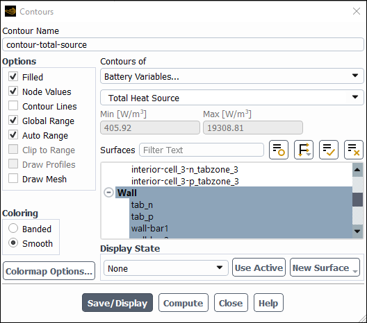
1. Enter contour-total-source for Contour Name.
2. Select Banded in the Coloring group box.
3. From the Contours of drop-down list, select Battery Variables... and Total Heat Source.
4. From the Surfaces selection list, select Wall.
5. Click Save/Display and close the Contours dialog box.
Figure 32.11: Total Heat Generation Rate
Save the case file (1P3S_battery_pack.cas.h5).
File → Write → Case...

32.5. Summary

This tutorial has demonstrated the use of the MSMD battery model to perform electrochemical and heat transfer simulations for battery packs. You have learned how to set up and solve the problem for the battery pack of the 1P3S configuration using the NTGK Battery submodel. You have also learned some of the postprocessing capabilities available in the MSMD battery model.