


This tutorial is divided into the following sections:
This tutorial is used to show how to set up a battery cell simulation in Ansys Fluent.
This tutorial demonstrates how to do the following:
Set up a battery cell simulation using the NTGK battery submodel
Perform the calculations for different battery discharge rates and compare the results using the postprocessing capabilities of Ansys Fluent
Use the reduced order method (ROM) in a battery simulation
Simulate a battery pulse discharge
Introduce external and internal short-circuits in a battery simulation
This tutorial is written with the assumption that you have completed the introductory tutorials found in this manual and that you are familiar with the Ansys Fluent outline view and ribbon structure. Some steps in the setup and solution procedure will not be shown explicitly.
The discharge behavior of a lithium-ion battery described in Kim’s paper [2] will be modeled in this tutorial. You will use the NTGK model. The battery is a 14.6 Ah LiMn2O4 cathode/graphite anode battery. The geometry of the battery cell is shown in Figure 31.1: Schematic of the Battery Cell Problem. You will study the battery’s behavior at different discharge rates.

For external and internal short-circuit treatment, you will consider an extreme case where external and internal short-circuits occur at the same time. You will simulate post-short-circuit battery processes. You can assume that the internal short is caused by a nail penetration occurring near the center of the battery.
The following sections describe the setup and solution steps for this tutorial:
Download the
battery_cell.zipfile here .Unzip
battery_cell.zipto your working directory.The mesh file
unit_battery.msh.h5can be found in the folder.Use the Fluent Launcher to start Ansys Fluent.
Select Solution in the top-left selection list to start Fluent in Solution Mode.
Select 3D under Dimension.
Enable Double Precision under Options.
Set Solver Processes to
1under Parallel (Local Machine).
Read the mesh file
unit_battery.msh.h5. File → Read →
Mesh...
File → Read →
Mesh...
When prompted, browse to the location of the
unit_battery.msh.h5and select the file.Once you read in the mesh, it is displayed in the embedded graphics windows.
The geometry is already in the correct scale. You don’t need to scale it.
Check the mesh.
Domain → Mesh
→ Check → Perform Mesh
Check
The following sections describe the setup steps for this tutorial:
In the Solver group of the General task page, enable a time-dependent calculation.
 Setup
→
Setup
→  General
→ Transient
General
→ TransientEnable the battery model.
Setup → Models
→ Battery Model Edit
EditIn the Battery Model dialog box, select Enable Battery Model.
The dialog box expands to display the battery model’s settings.
Once you enable the battery model, the Energy equation will be automatically enabled in order to solve for the temperature field.
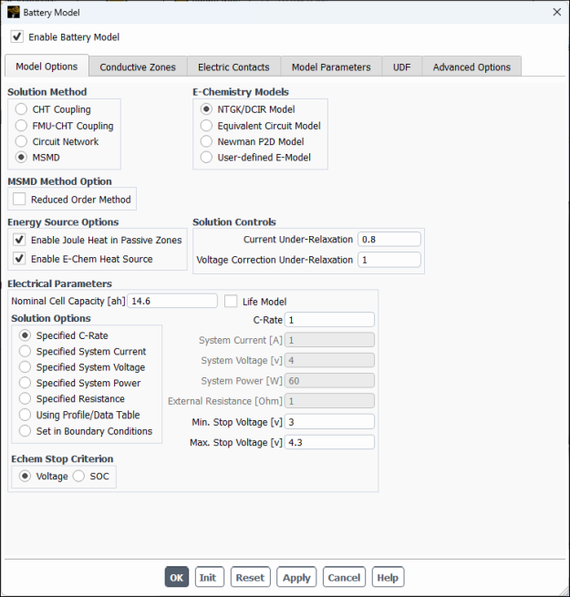
Under the Model Options tab (Figure 31.2: Model Options), configure the following battery operation conditions:
Ensure that MSMD is selected for Solution Method.
Under E-Chemistry Models, enable the NTGK/DCIR Model.
Under Electrical Parameters, retain the default value of
14.6 Ahfor Nominal Cell Capacity.Select Enable Joule heat in Passive Zones in the Energy Source Options group box.
Retain the default selection of Specified C-Rate and the value of
1for C-Rate.Retain the default value of
3 Vfor Min. Stop Voltage.
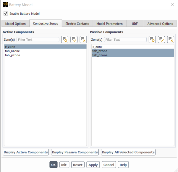
Under the Conductive Zones tab (Figure 31.3: Conductive Zones), configure the following settings:
Group
Control or List
Value or Selection
Active Components
Zone (s)
e-zone
Passive Components
Zone (s)
tab_nzone
tab_pzone
For this single cell case, there are no busbar zones. Electro-chemical reactions occur only in the active zone. Battery tabs are usually modeled as passive zones, in which the potential field is also solved.
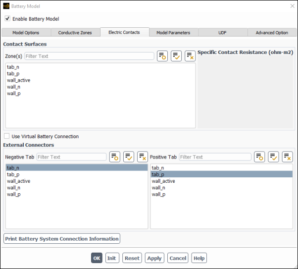
Under the Electric Contacts tab (Figure 31.4: Electric Contacts), configure the contact surface and external connector settings as follows:
Group
Control or List
Value or Selection
External Connectors
Negative Tab
tab_n
Positive Tab
tab_p
The corresponding current or voltage boundary condition will be applied to those boundaries automatically.
Under the Electric Contacts tab, you can also define extra contact resistance for each zone.
Click the button.
Ansys Fluent prints the battery connection information in the console window:
Battery Network Zone Information:
-------------------------------------
 Battery 1s1p
     Active zone:  e_zone

 Passive zone 0:
        tab_nzone
 Passive zone 1:
        tab_pzone
-------------------------------------
Number of battery series stages =1;  Number of batteries in parallel per series stage=1
****************END OF BATTERY CONNECTION INFO**************
Verify that the connection information is correct.
Under the Model Parameters tab, retain the default settings for Y and U coefficients.
Note:If in your case, Y and U functions are not in the same function form as in Kim’s paper, you need to modify the
cae_user.csource code file.For a given battery, you can perform a set of constant current discharging tests, and then use the battery's parameter estimation tool to obtain the Y and U functions.
Click to close the Battery Model dialog box.
In the background, Fluent automatically hooks all the necessary UDFs for the problem.
Click to close the Information dialog box.
Define the new e_material material for the battery’s cell, p_material for the positive tab, and n_material for the negative tab.
In the battery model, two transport equations are solved for the positive and negative potentials, respectively. To specify the electric conductivity of the active material you need to define the two electric conductivities, one for each potential field..
Create the electric material.
Physics → Materials
→ Create/Edit...
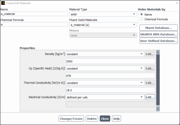
In the Create/Edit Materials dialog box, select solid from the Material Type drop-down list.
Enter
e_materialfor Name andefor Chemical Formula.Under Properties, set Density to
2092[kg/m3].Set Cp (Specific Heat) to
678[J/kg-K].Set Thermal Conductivity to
18.2[W/m-K].Select defined-per-uds from the Electrical Conductivity drop-down list.
In the UDS Diffusion Coefficients dialog box, specify the user-defined scalars.
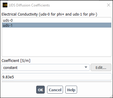
Select uds-0 in the User-Defined Scalar Diffusion list.
Retain constant from the Coefficient drop-down list.
Set Coefficient to
1.19e6.In a similar way, set uds-1 to
9.83e5and click OK to close the UDS Diffusion Coefficients dialog box.In the Question dialog box, click No to retain aluminum and add the new material (e_material) to the materials list.
Create a new material for the positive tab by modifying copper from the solid material database.
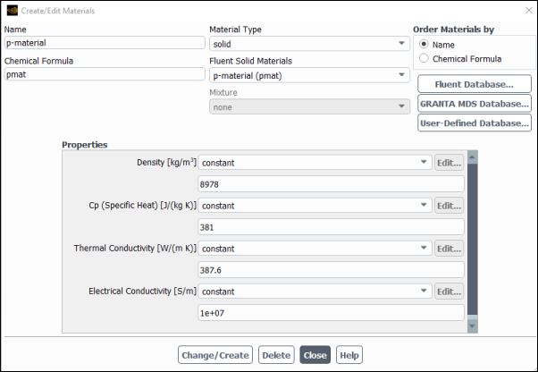
In the Create/Edit Materials dialog box, click .
In the Fluent Database Materials dialog box, make sure that solid is selected for Material Type.
Select
copperfrom Fluent Solids Materials and click and then Close.The Create/Edit Materials dialog box now displays the copied properties for
copper.Enter
p_materialfor Name andpmatfor Chemical Formula.Ensure constant is selected for Electrical Conductivity and enter
1.0e7.Click Change/Create.
In the Question dialog box, click Yes to overwrite copper.
The new material
(p_material)appears under Materials.
Create a new material for the negative tab with the same properties as the material for the positive tab.
Note: You do not need to create two different materials for the positive and negative tabs if the positive and negative tabs are made of the same material. In this tutorial, the two different tab materials with the same physical properties have been created for demonstration purposes only.
From Fluent Solid Materials drop-down list, select
p_material.Enter
n_materialfor Name andnmatfor Chemical Formula.Click .
In the Question dialog box, click No to retain p_material and add the new material (n_material) to the materials list.
Close the Create/Edit Materials dialog box.
Assign e_material to the cell zone, p_material to the positive tab and n_material to the negative tab.
Assign e_material to the e_zone zone.
Setup → Cell Zone
Conditions →  e_zone → Edit...
In the Solid dialog box, select
e_materialfrom the Material Name drop-down list.Click .
In a similar manner, assign p_material to tab_pzone and n_material to tab_nzone.
Define the thermal boundary conditions for all walls for the cell, and positive and negative tabs.
Set the convection boundary condition for wall_active.
Setup → Boundary
Conditions → Wall
wall_active → Edit...
In the Wall dialog box, under the Thermal tab, under Thermal Conditions, enable Convection.
Set Heat Transfer Coefficient to
5 [w/m2K].Retain the default value of
300 [K]for Free Stream Temperature.Click and close the Wall dialog box.
You do not need to change the settings under the UDS tab since the boundary conditions for the two UDS scalars have been set automatically when you defined the cell zone conditions.
Copy the boundary conditions for
wall_activetowall_pandwall_n. Setup → Boundary
Conditions →
wall_active Copy...
Make sure that wall_active is selected in the From Boundary Zone list.
Select wall_n and wall_p in the To Boundary Zone list.
Click Copy, click OK in the confirmation prompt, and close the Copy Conditions dialog box.
Turn off the flow and turbulence equations.
Solution → Controls
→ Equations...
In the Equations dialog box, deselect
FlowandTurbulencefrom the Equation selection list.Click .
Remove the convergence criteria to ensure that automatic convergence checking does not occur.
Solution → Reports
→ Residuals...
In the Residual Monitors dialog box, enable Show Advanced Options.
Select none from the Convergence Criterion drop-down list.
Click .
Create a surface report definition for the voltage at the positive tab.
Solution → Reports
→ Definitions → New
→ Surface Report → Area-Weighted
Average
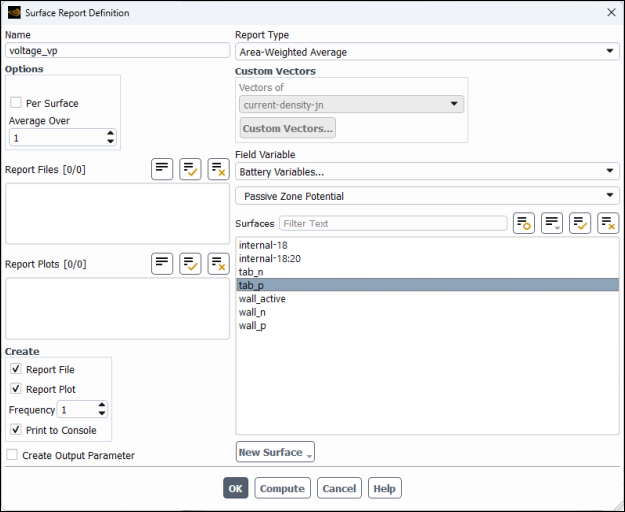
In the Surface Report Definition dialog box, enter
voltage_vpfor Name.Select Battery Variables... and Passive Zone Potential from the Field Variable drop-down lists.
From the Surfaces selection list, select tab_p.
In the Create group box, enable Report File, Report Plot and Print to Console.
Click to save the voltage_vp report definition and close the Surface Report Definition dialog box.
Rename the report output file.
Solution
→ Monitors → Report
Files → voltage_vp-rfile
Edit...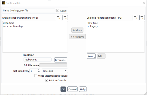
Enter
ntgk-1c.outfor File Name.Click to close the Edit Report File dialog box.
Modify the attributes of the plot axes.
Solution
→ Monitors → Report
Plots → voltage_vp-rplot
Edit...In the Edit Report Plot dialog box, under the Plot Window group box, click the button to open the Axes dialog box.
Select the X axis and set Precision to
0.Click .
Select the Y axis and set Precision to
2.Click and close the Axes dialog box.
Note: You must click Apply to save the modified settings for each axis.
Make sure that time-step is selected from the Get Data Every drop-down list.
Click OK to close the Edit Report Plot dialog box.
Create a volume report definition for the maximum temperature in the domain.
Solution → Reports
→ Definitions → New
→ Volume Report → Max...

In the Volume Report Definition dialog box, enter
max_tempfor Name.Select Temperature... and Static Temperature from the Field Variable drop-down lists.
From the Cell Zones selection list, select all zones.
In the Create group box, enable Report File, Report Plot and Print to Console.
Click to save the volume report definition settings and close the Volume Report Definition dialog box.
Rename the report output file.
Solution
→ Monitors → Report
Files → max_temp-rfile
Edit...Enter
max-temp-1c.outfor Output File Base Name.Click to close the Edit Report File dialog box.
Modify the axis attributes by setting the Precision to
0for the X axis and to2for the Y axes (in a manner similar to the surface plot definition).Click .
Save the case file (
unit_battery.cas.h5). File → Write
→ Case...
Initialize the field variables using the Standard Initialization method.
Solution →
Initialization
Retain the selection of the Standard method (Initialization group).
Click Initialize.
You do not need to modify Initial Values in the Solution Initialization task page, because these values are not used for initialization. The Ansys Fluent solver automatically computes the initial condition for UDS0 and UDS1.
Note: Warning messages are printed in the Fluent console informing you about interior zones between different solids. Such messages appear when two adjacent solid zones separated by an interior face type are using two different materials. The message suggests using the mesh/modify-zones/slit-interior-between-diff-solids text command to slit the interior zone between solid zones of differing materials to create a wall/wall-shadow interfaces. In general, the material property interpolation at wall/wall-shadow is more accurate if different materials are used at two sides of an interface. However, the battery model is implemented in such a way that both treatments are equivalent, and such messages could be ignored.
Run the simulation.
Solution → Run
Calculation
Set Time Step Size to
30seconds and No. of Time Steps to100.Click Calculate.
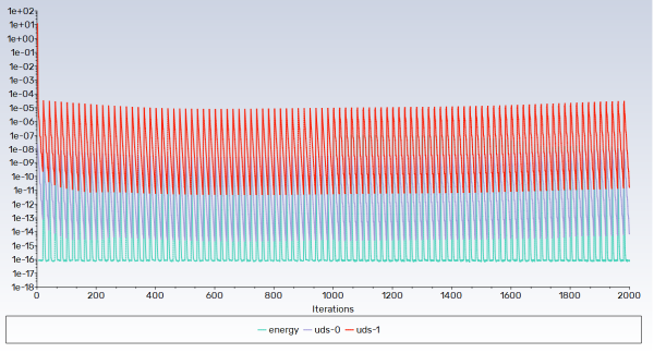
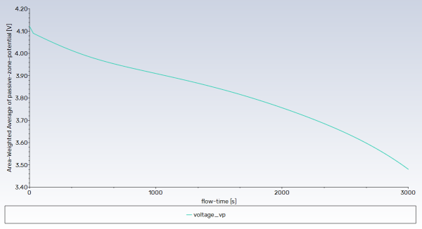
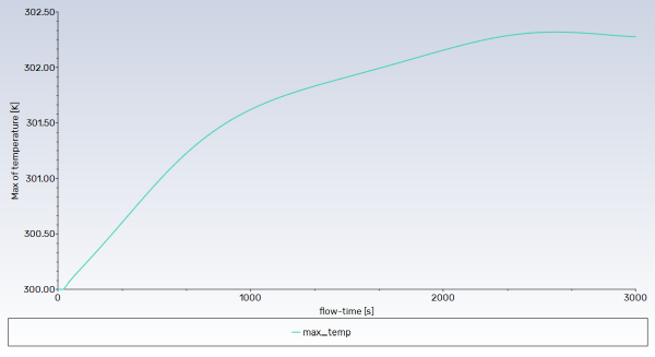
The residual plot, the report for voltage at the positive tab and the history of the maximum temperature in the domain are shown in Figure 31.5: Residual History of the Simulation, Figure 31.6: Report Plot of Discharge Curve at 1 C, and Figure 31.7: History of Maximum Temperature in the Domain, respectively.
Save the case and data files (
unit_battery.cas.h5andunit_battery.dat.h5). File → Write
→ Case & Data...
In this section, postprocessing capabilities for the MSMD battery model solution are demonstrated.
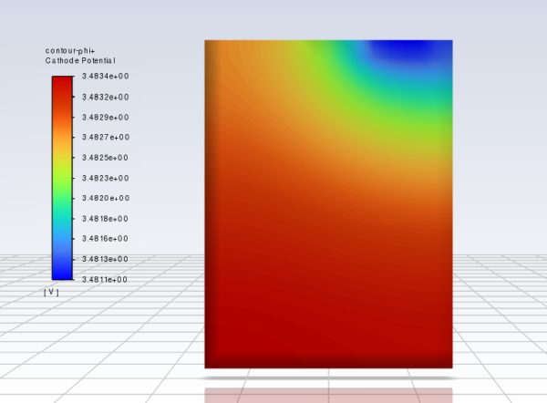
Display the contour plot of the phase potential for the positive electrode.
Results → Graphics
→ Contours → New...
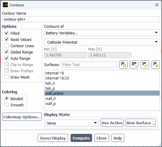
Enter
contour-phi+for Contour Name.Select Banded in the Coloring group box.
From the Contours of drop-down list, select Battery Variables... and Cathode Potential.
Click the button next to the Surfaces filter and from the drop-down list, select Surface Type (under Group by).
From the Surfaces selection list, under Wall, select wall_active.
Click and close the Contours dialog box.
Note: To change the precision for the colormap labels, click Colormap Options... to open the Colormap dialog box, and increase the value of Precision.
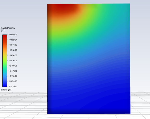
In a similar manner, display the contour plot of the phase potential for the negative electrode.
Results → Graphics
→ Contours → New...
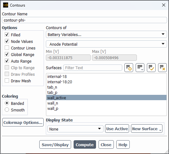
Enter
contour-phi-for Contour Name.Select Banded in the Coloring group box.
From the Contours of drop-down list, select Battery Variables... and Anode Potential.
From the Surfaces selection list, select wall_active.
Click and close the Contours dialog box.
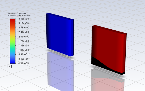
Display a contour plot of the phase potential in the passive zones
Results → Graphics
→ Contours → New...
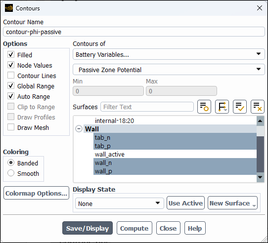
Enter
contour-phi-passivefor Contour Name.Select Banded in the Coloring group box.
From the Contours of drop-down list, select Battery Variables... and Passive Zone Potential.
From the Surfaces selection list, select tab_n, tab_p, wall_n, and wall_p.
Click and close the Contours dialog box.
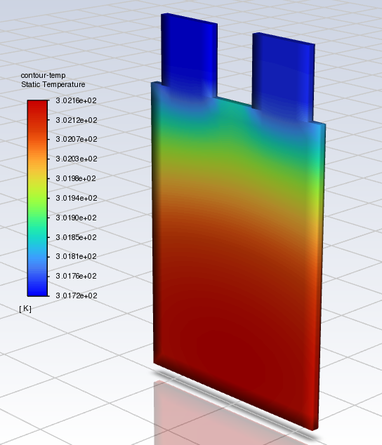
Display the contour plot of the temperature.
Results → Graphics
→ Contours → New...
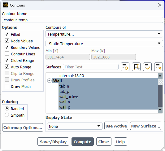
Enter
contour-tempfor Contour Name.Select Banded in the Coloring group box.
From the Contours of drop-down list, select Temperature... and Static Temperature.
Select Wall in the Surfaces selection list.
The surfaces listed under Wall are automatically selected in the Surfaces list.
Click and close the Contours dialog box.
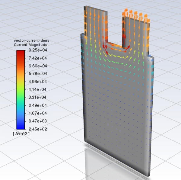
Display the vector plot of current density.
Results → Graphics
→ Vectors → New...
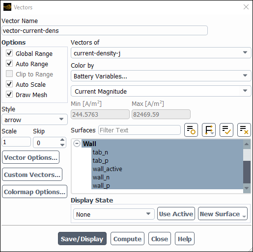
Enter
vector-current-densfor Vector Name.Select arrow from the Style drop-down list.
In the Vectors dialog box, select current-density-j from the Vectors of drop-down list.
Select Battery Variables... and Current Magnitude from the Color by drop-down list.
Click the button next to the Surfaces filter and from the drop-down list, select Surface Type (under Group by).
From the Surfaces selection list, select Wall.
In the Options group, enable Draw Mesh and in the Mesh Display dialog box, set the mesh display options as desired.
Click and close the Vectors dialog box.
Save the case file as
ntgk.cas.h5. You will use this saved case later to treat electric short-circuits.Repeat the simulation for the following charge rates and time steps:
C-Rate
Number of Time Steps
0.5 C
230
5 C
23
Make the following changes in the model’s settings:
Setup → Models
→ Battery Model
Edit...
In the Battery Model dialog box, under the Model Options tab, specify the value listed in the above table for the C-Rate.
Modify the output filename for the voltage_vp-rfile report file by entering
ntgk-for Output File Base Name in the corresponding Edit Report File dialog box, whereC-Rate.outC-Rateis the value of the battery discharge rate. (For example, for C-Rate = 0.5 C, you will enterntgk-0.5c.outfor the filename).Similarly, modify the output filename for max_temp-rfile by entering
max-temp-for Output File Base Name in the corresponding Edit Report File dialog box.C-Rate.outInitialize and run the solution for the number of the times steps specified in the above table.
Note: The Fluent solver will stop either after completing the specified number of time steps or when the Min. Stop Voltage condition is reached.
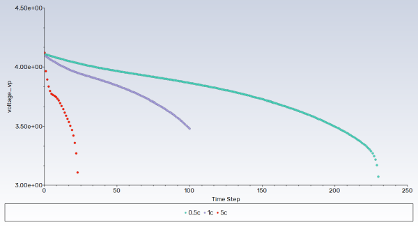
Display the discharge curves for the positive tab for the different discharge rates.
Open the Plot Data Sources dialog box.
Results → Plots
→ Data Sources...
Click Load File... to open the Select File dialog box.
Change the Files of type: drop-down filter to All Files (*), select
ntgk-0.5c.outand click .Deselect flow-time from the Y Axis Variables selection list.
Select voltage_vp in the Legend Names group box, enter
0.5cin the text box that populates below it and click .Do the same for
ntgk-1c.outandntgk-5c.outand change their legend entries accordingly.Enter
Discharge Ratefor the Legend Label in the Plot group box.Click Plot and close the Plot Data Sources dialog box.
Note: Use the Axes dialog box to set the precision for the plot axes.
The Figure 31.13: NTGK Model: Discharge Curves shows the discharge curves for different discharge rates in the function of time.
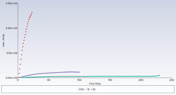
In a manner similar to the previous step, load the files
max-temp-0.5c.out,max-temp-1c.out, andmax-temp-5c.outand display the maximum temperature curves in the domain.Figure 31.14: NTGK Model: Maximum Temperature in the Domain shows the maximum temperature curves in the simulation for different discharge rates.
![]() Setup → Models →
Battery Model
Setup → Models →
Battery Model ![]() Edit...
Edit...
In the Battery Model dialog box, under E-Chemistry Models, select Equivalent Circuit Model.
Under Electrical Parameters, retain the default value of
14.6 Ahfor Nominal Cell Capacity.Retain the default selection of Specified C-Rate and enter
1for C-Rate.Under the Model Parameters tab, retain the battery specific parameters.
For a given battery, these model parameters can be obtained using the battery's HPPC testing data.
Click to apply the ECM battery model settings and close the Battery Model dialog box
Click in the Warning dialog box informing you that the re-initialization of the battery model is required.
In the Solution Initialization task page, click Initialize to re-initialize the field variables.
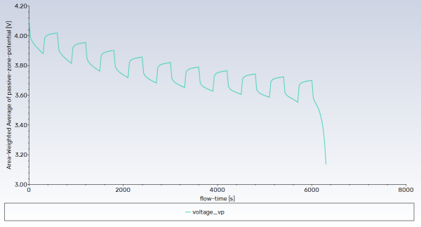
Simulate the battery pulse discharge by changing the battery operating conditions each time after running the calculation for five minutes.
In the Run Calculation task page, make sure that Time Step Size is set to 30, set Number of Time Steps to 10 and click Calculate.
Click to create new report definition files.
Once the calculation is complete, set C-Rate in the MSMD Battery Model dialog box to
0and run the calculation for 10 more time steps.Continue the simulation by alternating the value of C-Rate between 1 C and 0 C until, until the battery is fully discharged.
Note: Instead of doing this manually, you can use the Using Profile option in the MSMD Battery Model dialog box and load a profile file with specified C-rate fluctuations to drive the whole process. For more information about the usage of a profile file, refer to Specifying Battery Model Options in the Ansys Fluent User's Guide.
The battery pulse discharge is summarized in Figure 31.15: Battery Pulse Discharge.
You will use the ntgk.cas.h5 case file that you saved earlier
to illustrate how to use the ROM for time-efficient calculations. This section assumes that
you are already familiar with the Ansys Fluent battery model; only the steps related
specifically to using the ROM for problem solution are discussed here.
Read the NTGK model case file
ntgk.cas.h5.Initialize the problem.
In the Run Calculation task page, make sure that Time Step Size is set to 30, set Number of Time Steps to 3 and click Calculate.
Click in the Question dialog box when asked if you would like to append the new data to the existing file, and then click in the Warning dialog box to overwrite the existing file.
Once the calculation is complete, enable the ROM.
Setup → Models
→ Battery Model
Edit...
In the MSMD Method Option group box, select Reduced Order Method.
Set Number of Sub-Steps/Time Step to
10and click to close the Battery Model dialog box.
Re-run the simulation continuing from step 2 in Obtaining Solution.
The solution of the simulation using the ROM is significantly faster than when using the direct method without any changes in results.
You will again use the ntgk.cas.h5 case file that you saved
earlier to illustrate how to treat external and internal short-circuits in a battery
simulation. It is assumed that the battery is experiencing external and internal
short-circuit simultaneously. This extreme case will be used to demonstrate the problem
setup and postprocessing in a short simulation. This section assumes that you are already
familiar with the Ansys Fluent battery model, only the steps related to short simulation are
emphasized here.
Read the NTGK model case file
ntgk.cas.h5.Set up the external electric short-circuit.
Setup → Models
→ Battery Model
Edit...
In the Battery Model dialog box, under the Model Options tab, in the Solution Options group box, enable Specified Resistance.
For External Resistance, enter
0.5
                    Ohm
and click .
Set up the internal electric short-circuit in the center of the battery cell.
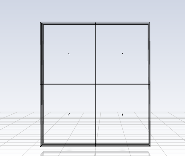
Mark the short-circuit zone shown in Figure 31.16: Internal Short Circuit Region Marked for Patching using a region register.
Solution → Cell
Registers New →
Region...
In the Region Register dialog box, enter the following values for Input Coordinates.
X Min
X Max
Y Min
Y Max
Z Min
Z Max
-0.01
0.01
-0.01
0.02
-1
1
Click Save/Display and close the Region Register dialog box.
Fluent reports in the console that 12 cells were marked for refinement.
Initialize the field variables using the standard initialization method.
Solution
→ Initialization
→ Initialize
Patch the internal short circuit zone with the short resistance value.
Solution
→ Initialization
→ Patch...
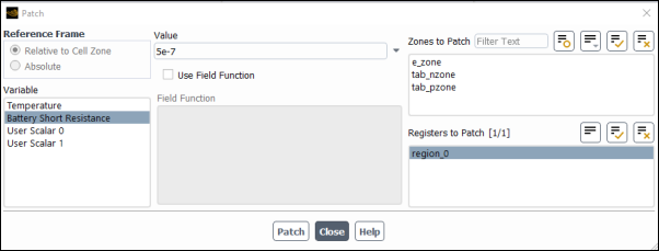
In the Patch dialog box, select Battery Short Resistance under Variable.
Select
region_0under Registers to Patch.For Value, enter
5.0e-7.Click Patch and close the Patch dialog box.
Save the case file (
ntgk_short_circuit.cas.h5). File → Write
→ Case...
Run the simulation for 5 seconds.
Solution → Run
Calculation
Set Time Step Size to
1second and No. of Time Steps to5.Click .
Save the case and data files (
ntgk_short_circuit.cas.h5andntgk_short_circuit.dat.h5). File → Write
→ Case & Data...
Compute the battery tab voltage
 . Results → Reports
→ Surface Integrals...
. Results → Reports
→ Surface Integrals...
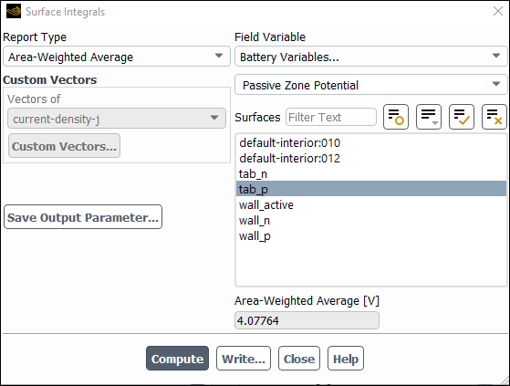
In the Surface Integrals dialog box, from the Report Type drop-down list, select Area-Weighted Average.
From the Field Variable drop-down lists, select Battery Variables... and Passive Zone Potential.
In the Surfaces filter, type
tto display surface names that begin with "t" and select tab_p from the selection list.Click and close the Surface Integrals dialog box.
The battery tab voltage of approximately 4.077 V is printed in the Area-Weighted Average field and in the Fluent console.
Compute the battery tab current
 . Results → Reports
→ Volume Integrals...
. Results → Reports
→ Volume Integrals...
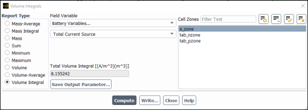
In the Report Type group box, select Volume Integrals.
From the Field Variable drop-down lists, select Battery Variables... and Total Current Source.
From the Cell Zones selection list, select
e_zone.Click Compute and close the Volume Integrals dialog box.
Fluent reports in the Total Volume Integral field and in the console that the total volume integral for the volumetric current source is approximately 8.155 A.
The computed values of the battery tab current and voltage satisfy the tab boundary condition
 .
.
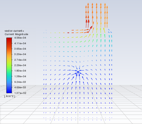
Display the vector plot of current at the positive and negative current collectors.
Results → Graphics
→ Vectors → New...
Enter
vector-current+for Vector Name.Select arrow from the Style drop-down list.
In the Vectors dialog box, select current-density-jp from the Vectors of drop-down list.
Select Battery Variables... and Current Magnitude from the Color by drop-down lists.
From the Surfaces selection list, select Wall.
The surfaces of the "wall" type are automatically selected in the Surfaces list.
Click .
The plot shows the vector plot of electric current flow in the positive current collector of the battery cell.
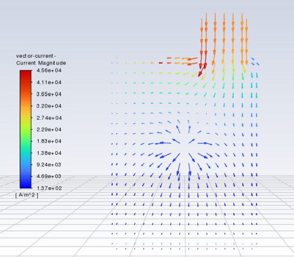
In a similar manner, display the current for the negative current collector by selecting current-density-jn from the Vectors of drop-down list.
The plot shows the vector plots of electric current flow in the negative current collector of the battery cell. These plots clearly show that besides providing tab current, short current flows from positive electrode to the negative electrode through the short area.
Close the Vectors dialog box.
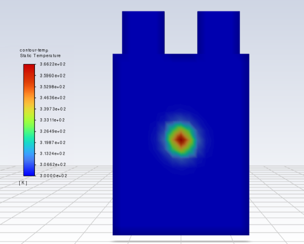
Display the contour plot of the temperature as you did previously.
Results → Graphics
→ Contours
→ contour-temp
DisplayFigure 31.19: Contour Plot of Temperature shows a temperature hotspot in the internal shorted area of the battery cell.
Check for different electric current flow rates in the manner described in step 2.
Results → Reports
→ Volume Integrals...
Generate volume integral reports for the field variables listed in the table below.
Field Variable
Notation
Reported Value
Short Current Source

-15.843 A
ECHEM Current Source

23.999 A
Verify that the total produced electric current equals to the sum of tab and short current, that is
 .
.
Check for different types of heat generation rates.
As you did for the current source reports, generate reports for the field variables listed in the table below.
Field Variable
Notation
Reported Value
Joule Heat Source

0 W
Echem Heat Source

1.092 W
Short-Circuit Heat Source

64.607 W
Total Heat Source

65.699 W
Verify that the total heat generation rate is the sum of different contributions, that is
 .
.
Save the case file (
ntgk_short_circuit.cas.h5). File → Write
→ Case...
Note that, as battery's temperature increases, thermal runaway may occur. If thermal runaway starts, some undesirable exothermic decomposition reactions will occur. For thermal runaway simulations, the default electrochemistry model cannot be used. Short treatment can only capture the thermal ramp-up process before the onset of thermal runaway.
In this tutorial, you studied how to solve a battery cell problem using the NTGK submodel with the default settings. You then used the ROM to speed up the computation time of the battery model simulation. In addition, you learned how to use the MSMD model capability to treat external and internal short-circuits.
For more information about using the Dual-Potential MSMD Battery model, see the Ansys Fluent User's and Theory Guides.
The battery cell cross-section is shown in the figure below.
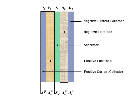
You can estimate the material properties for your battery cell using the following correlations:
For density
 , heat capacity
  , and thermal conductivity
  :
:where
 is the effective property value of a material property (such as density,
heat capacity, or thermal conductivity),
is the effective property value of a material property (such as density,
heat capacity, or thermal conductivity),  is the thickness. The subscripts
  ,
,  , and
, and  refer to current collector, electrode, and separator, respectively. The
superscripts
refer to current collector, electrode, and separator, respectively. The
superscripts  and
and  refer to positive and negative, respectively.
For electric conductivity
 :
:


The material properties are taken from Kim’s papers [2] and [1]. The computed material properties for the battery cell presented in the tutorial are shown in the table below.
|
Zone |
|
|
|
|
|
Total |
|---|---|---|---|---|---|---|
|
|
20 |
150 |
12 |
145 |
10 |
322 |
|
|
2700 |
1500 |
1200 |
2500 |
8960 |
2092 |
|
|
900 |
700 |
700 |
700 |
385 |
678 |
|
|
238 |
5 |
1 |
5 |
398 |
18.2 |
|
|
3.83e7 |
13.9 |
100 |
6.33e7 |
|


U. S. Kim et al, "Effect of electrode configuration on the thermal behavior of a lithium-polymer battery", Journal of Power Sources, Volume 180 (2), pages 909-916, 2008.
U. S. Kim, et al., "Modeling the Dependence of the Discharge Behavior of a Lithium-Ion Battery on the Environmental Temperature", J. of Electrochemical Soc., Volume 158 (5), pages A611-A618, 2011.