The following sections of this chapter are:
In this tutorial, you will compute rime ice accretion using a fully coupled unsteady approach, where the air and droplet solvers run in time-accurate mode as the grid geometry gets updated at each time step with ice accretion. Since unsteady solutions are expensive, the grid is coarse with no boundary layer resolution. The grid is acceptable for inviscid calculations and can be used with the Rime ice model as it does not require a viscous flow solution.
The airfoil is assigned a pitching and plunging motion that approximates the motion of a helicopter blade section during forward-flight. This motion is assigned using the Rigid Mesh Motion technique, where the entire mesh moves without any deformation. This greatly saves computational time by not solving for mesh deformation during the unsteady simulation process.
To provide a good initial solution to the unsteady problem, steady-state flow and droplet solutions will be obtained on the clean airfoil.
Create a new project using File → New project or the New project icon. Select the metric units system.
Create a new run using File → New run or the new run icon. Select FENSAP as the flow solver. Keep the default run name, FENSAP.
Download the
6_Unsteady_Advanced.zipfile here .Unzip
6_Unsteady_Advanced.zipto your working directory.Double-click the grid icon to assign the grid file. Select the grid file naca0012_inviscid provided by ANSYS in the tutorials subdirectory ../workshop_input_files/Input_Grid/Multiphase.
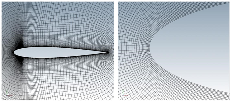
The grid is shown in the figure below. This grid is similar to the one used in the introductory tutorials section, but coarser in the normal direction near the wall, and therefore it is not suited for viscous calculations.
Double-click the config icon. A new window pops up to enable the selection of the FENSAP input parameters.
In the Momentum equations box, choose the Euler option (inviscid flow) and keep the Full PDE option in the Energy equation box. The prescribed motion of the airfoil generates work, therefore the air flow energy equation should be activated.
Go to the Conditions panel. Enter the Reference conditions for air:
Characteristic length 0.5334mAir velocity 102.8m/sAir static pressure 100000PaAir static temperature 241.49K (-31.66°C)In the Initial solution tab, select the Velocity angles option. Set the Angle of attack value to
4degrees.Go to the Boundaries panel. Click the BC_1000 family and select the Riemann option in the Type box. Click the Import reference conditions button. Verify that the three velocity components correspond to the imposed angle of attack.
Note: The Riemann invariants based on far field conditions permit the grid nodes of BC_1000 to seamlessly switch between inflow/outflow states, which is a necessity when the entire grid is set to pitch and plunge.
The wall boundaries 2001, 2002, 2003, should be set to Slip condition. No other adjustment is possible in inviscid flows.
Skip the Solver panel. The default CFL setting (100) and the default number of iterations (250) will be sufficient to converge the residuals to approximately 1e-10. Uncheck the Use variable relaxation option.
Go to the Out panel. Choose Solution every
20iterations in the Overwrite mode. Enable lift and drag computation in the Forces box by choosing Drag direction based on inlet BC. Set the Reference area to0.28451556m2 which is the planform area of the airfoil in this grid.Run this calculation on
4processors, if possible.Next, obtain a steady-state droplet solution. Create a new DROP3D run, and drag & drop the config icon of the FENSAP run onto the config of the DROP3D run.
In the Conditions panel, set the Liquid Water Content to
5.0g/m3. The LWC here is set intentionally high in order to accrete a sizeable amount of ice in a short period of time. The following unsteady calculation will be kept short in order to save execution time and disk space.The rest of the reference conditions are copied from the FENSAP run.
In the Boundaries panel, click the Inlet (BC_1000) and click Import reference conditions to copy the value of the Liquid Water Content.
Run the calculation on
4CPUs if possible.
Create a new run within the same project. Choose FENSAP as the solver. You can name the run
Multiphase.Drag & drop the config icon of the DROP3D run onto the config icon of this new run.
Go to the Model panel. In the Physical model box, choose Air + Droplets. This enables the airflow and droplet coupled solution mode. Note that the coupling is one way, meaning airflow affects the droplets but not the other way around.
Set the Momentum Equations to Euler as it was done for the initial flow calculation.
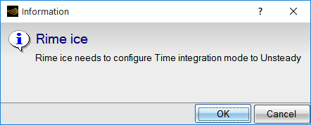
Choose the Rime option in the Icing model box near the bottom of the panel. A dialog box will appear prompting to enable the unsteady mode. Click to accept.
Keep the default ice density value.
Go to the Conditions panel. Set the Liquid Water Content to
5.0g/m3 in the Droplets reference conditions section. This unsteady calculation should begin with the steady-state flow and droplet solutions computed in the previous steps. To do this, select the Solution restart option in the Initial solution tab. Select the soln and droplet files produced in the two previous runs of this tutorial.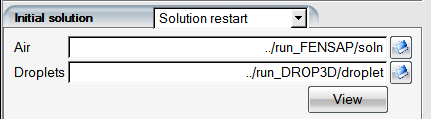
Go to the Boundaries panel and click the Inlet (BC_1000). Make sure it is set to Riemann as the BC Type, so that the inflow/outflow state of the boundary nodes can adapt automatically to the motion of the grid. Click button to make sure the droplet conditions are set as well. Note that Riemann invariants are used to resolve the air flow boundary conditions only. Droplets use the standard far field algorithm when air is set as Riemann.
Go to the Solver panel and select the Unsteady – Dual time stepping in the Time integration tab.
Set the CFL number to
50for both the flow and the droplet equations. The CFL number is used for the inner iterations of each physical time step, in order to converge the non-linear problem better. You should set the CFL number of both flow and droplet equations the same here so that both systems converge at the same pace. Set the value of Max. pseudo time iterations to4dual time integrations within each physical time step.In the next step, the frequency of the pitching and plunging motion will be set as 0.5 Hz. This is about 10 times less than a typical helicopter blade. This setting is used in this tutorial to be able to keep the unsteady time step high. It is recommended to resolve a period of motion with a decent temporal resolution to maintain time accuracy of an unsteady run. In this example, 200 time steps are used for one period, which requires a time step of 0.01 seconds.
Set the Time step to
0.01seconds and the Total time to10seconds.Select the Streamline upwind (SU) artificial viscosity scheme and set its Cross-wind dissipation to
1e-7and its order to100%, second order.Go to the Out panel. Save the Solution every
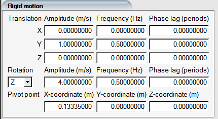
4iterations and choose Do not overwrite. This will save numbered grid and solution files every 0.04 seconds, which could be used to animate the motion of the airfoil real-time at 25 frames per second.In the same Out panel, set the ALE mode to Rigid motion. A new table of cyclic motion parameters will appear that defines the motion of the entire grid. The motion is broken down as translation and rotation about a given axis. Both modes of motion are governed by the sine trigonometric function. The translation mode assigns the grid velocity. Without a phase lag, the velocity in a given coordinate starts at 0 m/s at t = 0 and reaches its maximum value at quarter-period. By using a phase lag of 0.25 periods, the sine function can be converted to the cosine function to start the motion at the maximum speed at t = 0. The rotation mode uses the actual value of the rotation in degrees, relative to the original orientation of the grid. Following the sine function, at t = 0, the grid will be at 0 degrees, and at quarter-period it will have been rotated to the max amplitude of the rotation. To invert the motion, a negative amplitude can be entered, or alternatively the phase lag can be adjusted appropriately.
In this tutorial the amplitudes of the pitching and plunging motions will be set to
4degrees and1m/s, respectively. The flapping motion occurs along the Y axis, therefore set the flapping velocity amplitude to1m/s for the Y coordinate with a frequency of0.5Hz. The speed is set low in order to keep the airfoil in the viewing panel when animating the solutions in Viewmerical. This is a side effect of entering a low flapping frequency. The initial position of the blade is at its lowest, meaning that the translational velocity is 0 at t = 0. Therefore no phase lag is to be entered for the Y translation.Next, the rotation parameters need to be set for the pitching motion. Change the axis to Z, the amplitude to
4degrees and the frequency to 0.5 Hz. At t = 0, the airfoil is at its nominal angle of attack with a rotation of 0 degrees, meaning that no phase lag is to be set for the rotation either. The Pivot point will be set at the aerodynamic center of the airfoil, which is at X = 0.13335 m.The rotation follows the right-hand rule. In this grid the Z axis points “out of the screen” and a positive rotation will pitch the airfoil down, reducing the angle of attack.
The final Rigid motion parameter settings should look like this:
In the Forces menu, choose Drag direction based on inlet BC option, the Positive lift direction as +Y, and the Reference area to
0.28451556m2. The lift and drag curves in the Graphs panel will show the effect of motion on the aerodynamic forces experienced by the airfoil.Run this calculation on
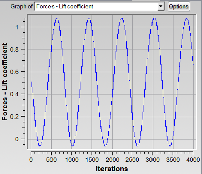
4or more processors, if possible.In the Graphs panel, switch to Lift coefficient in order to monitor its time-history. Every 800 iterations make up a period.
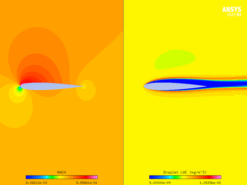
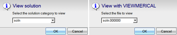
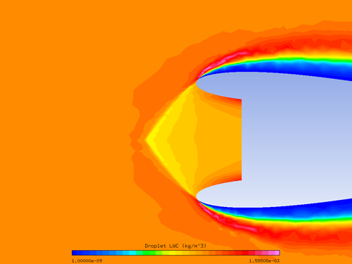
Upon completion, click the button in the Execution panel to visualize the flow and the droplet solutions on the displaced grid after 10 seconds of icing. After clicking View, choose soln category to access the menu for the air solution files. Next, choose soln.000000 from the list of air solution files. Loading the numbered solution files will automatically load the numbered grid files that have been modified with motion and ice surface displacement.
In the Data panel of Viewmerical, the solution files can be cycled using the slider bar. Doing so will display the grid and the solution at that step. The
 button can automatically cycle through the files. Align the view
with Z axis and zoom in to see the airfoil in motion.
button can automatically cycle through the files. Align the view
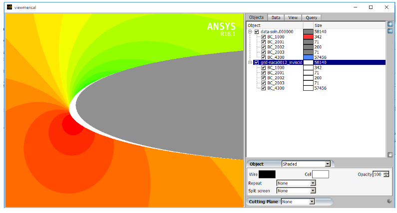
with Z axis and zoom in to see the airfoil in motion.To see the ice shape, move the slider bar all the way to the right to display the final grid at 10 seconds. Go back to the Objects panel, and by clicking the
 button on the top right, add the original grid
naca0012_inviscid. Choosing this second grid object in the list,
switch the display to Shaded and set the Cell
color to white. With static pressure displayed in the first object, the view should look
like this:
button on the top right, add the original grid
naca0012_inviscid. Choosing this second grid object in the list,
switch the display to Shaded and set the Cell
color to white. With static pressure displayed in the first object, the view should look
like this: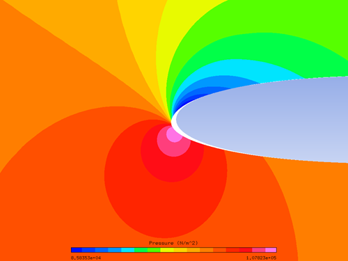
Screens covering the intakes of engines are prone to icing just as much as any other component that is exposed to incoming free stream air. Due to thin wire diameters that are in the order of a millimeter or less, screens have a high collection efficiency and they can ice quite rapidly. Screen icing can cause blockage and engine performance loss, which is an added burden on an aircraft which may already be suffering from icing effects like increased drag and stall speeds.
This tutorial demonstrates the screen icing model on a 2D Nacelle with a curved screen. You are invited to read Screen Models in the FENSAP-ICE User Manual for more information on screens. The first part of this tutorial sets up a steady-state airflow and droplet calculation to be used as the starting point for the unsteady simulation with icing carried out in the second part.
Create a new project using File → New project or the New project icon. Name the project
Screen-Ice. Select the metric units system.Create a new run using File → New run or the new run icon. Select FENSAP as the flow solver.
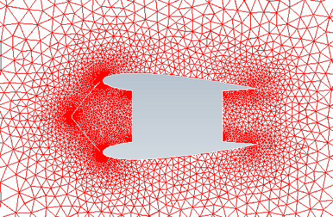
Double-click the grid icon to assign the grid file. Select the grid file grid_screen_v2 provided by Ansys in the tutorials subdirectory ../workshop_input_files/Input_Grid/Screen. The grid is shown in the figure below. The geometry is a 2D-Nacelle with a curved screen placed in-front of the intake.
Double-click the config icon. A new window opens to enable the selection of the FENSAP input parameters.
Keep the Navier-Stokes (viscous flow) and the Full PDE options. Select the Spalart-Allmaras turbulence model with an Eddy/laminar viscosity ratio value of
1e-5.Go to the Conditions panel. Enter the Reference conditions for air:
Characteristic length 0.5mAir velocity 100m/sAir static pressure 101325PaAir static temperature 265K (-8.15°C)In the Initial solution box select the Velocity angles option and keep them 0.
Go to the Boundaries panel.
Click the BC_1000 family and select the Supersonic or far field option in the Type tab. Click the button. Verify that the three Velocity components correspond to the values specified in the initial conditions.
Click the BC_1001 family and select the Mass flow option in the Type tab. Set the Static temperature and Mass flow rate to
450K (176.85°C) and8kg/s respectively. Alpha and Beta should be set to0.All wall boundaries should remain as No-slip with Heat flux set to
0(adiabatic walls).Click the BC_3000 family and select the Mass flow option in the Type tab. Set the Mass flow rate to
8kg/s.Click the BC_6000 family and select Screen in the Type tab. Set the Wire diameter to
0.001m and the Wire spacing to0.02m. In the Screen mode tab under Screen Model, select the Brundrett model to compute the pressure variation across the screen.Note: The screen boundary is disconnected from the nacelle walls. The unsteady screen icing simulation will also build rime ice on the walls and will deform the mesh.
Go to the Solver panel. Keep the CFL number at
100and set the Maximum number of time steps to600. Enable the Use variable relaxation option, which should be used when there are mass flow exits and keep the default settings provided in the configuration box that appears.Change the Crosswind dissipation to
1e-6, which is better for coarse grids.Go to the Out panel and set it to write the Solution every
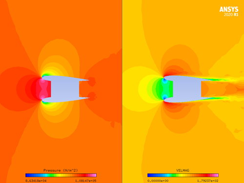
20iterations.Run this calculation on
4processors, if possible.Figure 6.5: Screens Extract Momentum from the Flow Due to the Friction over the Wires, Reducing the Total Pressure Across Them
Create a new run using File → New run or the new run icon. Select DROP3D as the flow solver.
Drag and drop the config icon of the previous FENSAP run onto the config icon of this DROP3D run to copy the reference and boundary conditions from the flow solution.
For this tutorial, the default values of free stream LWC (1 g/m3) and MVD (20 microns) are retained. Do not modify the reference and boundary conditions that have been automatically assigned by the drag & drop operation.
Go to the Boundaries panel.
Click the BC_1001 family. Set the Liquid Water Content to zero. This is the engine exhaust and no droplets are supposed to exist here. Uncheck the velocity components for this boundary so that they are set to values of air velocity at this inlet. This is recommended for internal inlets where the velocity to apply to droplets is not always obvious.
Click the button at the bottom of the panel to go to the Execution environment. In the Settings panel, set the Number of CPUs to
4, if possible.Click the menu button to start the calculations. The progress of the calculations can be monitored in the Execution panel.
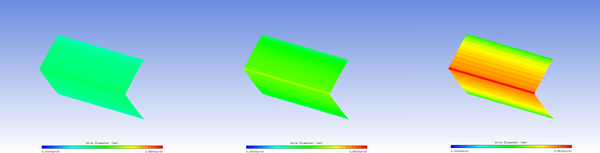
The screen will catch some of the droplets and reduce the LWC across. In icing conditions, the LWC caught by the screen will form ice and increase the wire diameters. The changes to the wire diameters are local, meaning it may be different based on the location on the screen.
Create a new run using File → New run or the new run icon. Select FENSAP as the flow solver. You can name this run
SCREEN_ICING.Drag and drop the config icon from the FENSAP run onto this one.
Double-click the config icon. In the Model panel, change the Physical model to Air + Droplets.
In the Icing model box select the Rime ice option. The application prompts you via a message window to enable the unsteady mode. Click the button.
The Conditions panel should contain the drag & drop reference values from the previous FENSAP steady state run. Keep these parameters as they are.
The initial conditions will be set to the steady-state air and droplet flow solutions obtained in the previous sections. Therefore, in the Initial solution tab, select the Solution restart option.
Browse and upload the airflow solution file soln of Steady-State Flow. Repeat the operation to upload the droplet solution file droplet from Steady-State Droplet Flow.
Go to the Boundaries panel.
Click the BC_1000 family and click the Import reference conditions button to set the droplet conditions correctly.
Click the BC_1001 family. Set Liquid Water Content to
0and clear the velocity components of the droplets.No changes to the wall boundaries are required.
Click the BC_3000 family and change the Type to Subsonic which specifies the pressure. When using screen icing, which is an unsteady process, it is not correct to use a mass flow exit. As the screen gets iced and starts to block the flow, the mass flow requirement cannot be satisfied exactly. Therefore, the pressure at this exit should be specified, which can be obtained from the restart solution. Set it to
105054.258Pa as determined in the airflow restart solution.Click the BC_6000 family. The screen settings should be carried over automatically with the drag and drop operation.
Note: Icing can only be enabled on screens if the time integration is set to unsteady in the Solver panel. This is automatically done when the icing model is enabled in the Model panel.
Go to the Solver panel. Change the Time Integration mode to Unsteady – Dual time stepping. Set the CFL number to
100for the flow with a Max. pseudo time iterations to2. Set the Time step to0.1s for a Total time of60s. Keep the CFL number for droplets at20.Note: The CFL numbers of flow and droplets do not have to be identical, but they should be in the same order of magnitude.
Go to the Out panel. Choose Solution every 100 iterations in Do Not Overwrite mode. This produces numbered solution files, for every 10 seconds.
Run this calculation on
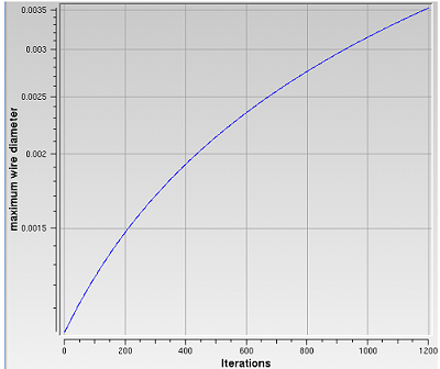
4processors, if possible.The change in maximum wire diameter can be observed in the Graphs panel, by choosing the maximum wire diameter graph.
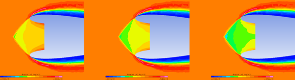
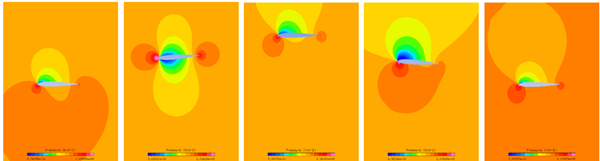
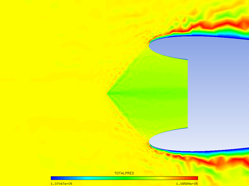
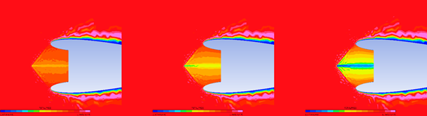
Click the button and launch Viewmerical to load the numbered soln and droplet files to see how the flow field changes in time with the effect of screen and surface icing. The plots below can be generated by sliding the Step bar in the Data panel from
0to600.Figure 6.8: Increase in Total Pressure Loss Across the Screen as Ice Accretes with Time (T=0.0s, T=30s, T=60s)
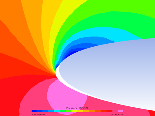
Finally, to see the shape of the ice accreted on the nacelle lips, click the + sign on the Object panel of Viewmerical and add the original grid_screen_v2 that should be available in the main project directory. Set this grid’s display mode to Colored and set its Cell coloring to white. Zoom in on the upper lip. With Pressure being displayed for the unsteady solution at step 600, the view should look like this: