For icing calculations, the unsteady air-droplets model introduced in Two-Phase Flows: Coupling Flow and Droplets is complemented by the Messinger model to compute accretion speed and to displace the surface grid in time.
The resulting system of coupled equations can be solved for inviscid (Euler equation) or viscous (Navier-Stokes) flows. For rime ice accretion, inviscid flow with constant total enthalpy is sufficient to guarantee accurate results. For glaze ice, however, the viscous equations should be complemented by the one-equation turbulence model to predict accurate shear stresses and by the full energy equation to compute heat fluxes on the walls.
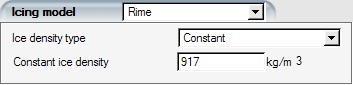
In the Model panel select Rime to activate rime ice growth in the Icing model section.
At very low temperatures, droplets impinging on the surface freeze on impact and therefore contribute directly to ice formation. This assumption represents a simple mass balance between droplets impingement and ice accretion:

where  is the rate of ice accretion in kg/m2s.
The surface displacement vector
is the rate of ice accretion in kg/m2s.
The surface displacement vector  is computed from the accretion speed (always normal to the iced
surface):
is computed from the accretion speed (always normal to the iced
surface):

as

where  is the ice density and
  is the physical time step. The accretion speed is imposed as
boundary conditions to the diphasic and mesh deformation models.
is the physical time step. The accretion speed is imposed as
boundary conditions to the diphasic and mesh deformation models.
The ice density can be set either to Constant (default 917 kg/m3) or computed using Macklin formula:

for 0.2 < RM < 170, where

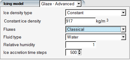
Select Glaze - Advanced to activate glaze icing.
This model couples the flow and droplets equations in time with the glaze icing
model of FENSAP-ICE, described in ICE3D - Ice Accretion and Water Runback, which solves
for local water film height (h), temperature (T) and accretion rate of ice
( ). As for the rime icing model (See Rime Ice), the accretion speed is obtained directly from
the ice accretion rate and used as input to displace the iced surface in time in the
ALE formulation.
). As for the rime icing model (See Rime Ice), the accretion speed is obtained directly from
the ice accretion rate and used as input to displace the iced surface in time in the
ALE formulation.
The ice density can be set either to Constant (default 917 kg/m3) or computed using the Macklin formula.
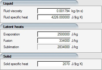
The heat fluxes are computed by FENSAP at each physical time step. They are then directly affected by ice growth in time and the resulting changes in boundary layer characteristics. Choose between Gresho heat flux type (default) and the Classical (k·dT/dn) form. Water and ice are the default media, and their thermodynamic characteristics are automatically supplied to FENSAP-ICE-Unsteady.
The Relative humidity is expressed from 0 (0%) to 1 (100%, or default). For clouds, this value should be set to 1 (or 100%). Otherwise, enter the relative humidity of the icing tunnel, as determined during the experiment.
Since icing is an unsteady phenomenon, the different solutions should be saved at fixed intervals in time, and in separate files numbered by the iteration number. These include:
The flow solution file
The droplets solution file
The displaced grid in function of the ice shape
The CAD of the iced geometry saved in ICEM CFD TETIN format
The CAD of the iced geometry saved in .stl format