


The conservation of mass and momentum can be defined from the one fluid formulation for multiphase flow:

where the subscript  refers to gas and
  to droplet particles. The right-hand side (
 ) terms include the effects of air on droplets and of droplets on
air.
) terms include the effects of air on droplets and of droplets on
air.

In this equation, the time derivative terms account for mesh displacement using the Arbitrary Lagrangian Eulerian (ALE) formulation.
During in-flight icing conditions, the droplets volume fraction (ag) is of the order of 10-6. Therefore the air volume fraction (ap) can be considered constant and equal to one and the air-droplets flow is viewed as a dilute gas particle system, where only the effects of air on droplets are accounted for. The resulting equations for air:

and droplets:

correspond in essence to the governing equations of the icing codes FENSAP, for air, and DROP3D, for droplets impingement. The main difference in this work is that the one-way-coupled equations are solved together in time.
Select Air + Droplets under Physical model to solve for the coupled flow and droplets equations as a multiphase flow.
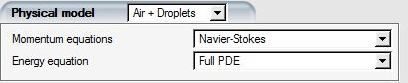
In the case of unsteady calculations, the Energy equation option should be set to Full PDE mode. Transition to turbulence or sand-grain roughness can be imposed as well.
To improve the performance of the iterative matrix solver, the terms associated with the temporal operator of the equations can be added to the Jacobian matrix (these terms do not affect the residuals).
The addition of these terms, proportional to  , increases the diagonal dominance of the Jacobian matrix and
improves the convergence of the iterative solver. The solution is then advanced in
time until the time derivative terms become zero, or the flow field reaches
steady-state.
, increases the diagonal dominance of the Jacobian matrix and
improves the convergence of the iterative solver. The solution is then advanced in
time until the time derivative terms become zero, or the flow field reaches
steady-state.
The choice of the local time step, for an element, is based on the stability
analysis of the explicit-Euler centered finite difference scheme, which provides a
maximum theoretical  . The time step is then selected as:

The solution is advanced in time, with a  that varies from one cell to another, until steady-state is
reached. Only one Newton iteration is performed to linearize the system at each time
step. The linear matrix system is solved using a GMRES approach.
that varies from one cell to another, until steady-state is
reached. Only one Newton iteration is performed to linearize the system at each time
step. The linear matrix system is solved using a GMRES approach.
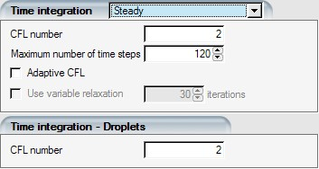
To select this option, click Steady. Enter the CFL number for air (from 50 to 1,000, default 100) and for droplets (between 1 and 50, default 2), and the maximum number of time steps. The calculation ends if either the maximum number of time steps or the convergence residual level criteria have been reached.
Tip: Reduce the CFL number if convergence problems are encountered.
Two time stepping schemes are available for unsteady time-accurate simulations.
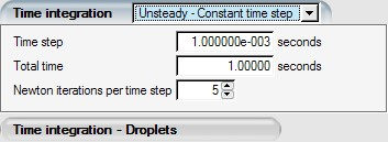
Select to solve for an unsteady flow using a constant time step. Set the time step and the total solution time, both in seconds. The solution is advanced in time using a second-order Gear scheme. The non-linear governing equations are linearized by performing, at each time step, a given number of Newton linearization loops (default 5). The solver then moves to the next time step if either the number of Newton iteration per time step is reached or, the convergence residual level criteria is satisfied. The calculation stops at the end of the total time.
Note: The convergence of the GMRES solver is closely linked to the time step, since the time derivative term affects the diagonal dominance of the linear matrix system. Reduce the time step if the GMRES solver is not converging more than two orders of magnitude.
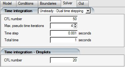
Select to solve for an unsteady flow using a dual time approach. Set the physical time step and the total solution time, both in seconds. The solution advances in physical time using a second-order Gear scheme. At each physical time step, the non-linear governing equations are converged in pseudo-time using a local time stepping technique with a constant CFL number. Make sure to perform enough pseudo-time iterations (default 4) to ensure solver convergence. The calculation stops at the end of the total physical time. It is important to use the same CFL number for airflow and droplet calculations so that they advance in similar fashion during each physical time step. For example, if the DROP3D CFL number is lower than the CFL number of the air flow, the droplet solution may not converge sufficiently and calculation can be compromised.
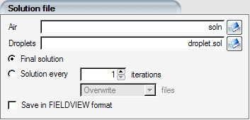
Even if the flow and droplets solutions are coupled, their solutions will be saved in two separate files. Enter the name of the airflow solution file in the Air box, and the droplets solution file in the Droplets box. Select Overwrite to save solutions every N iterations in the same files. Select Do not overwrite to save solutions every X iterations in different numbered files.