


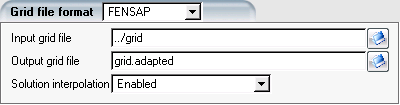
Solution interpolation permits you to choose if an interpolated solution file is written along the adapted grid. Not writing the solution file permits you to save disk space.
Disabled: No output solution file.
: (Default) Interpolated solution file is written.
Subset of fields - for restarts: A minimum amount of datafields are written to the output file. This is useful to reduce the output file size, while retaining the capability to use the file as a restart.
Note: Available for Fluent only (V, P, T, TKE, SDE fields are only written when this option is selected).
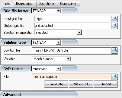
The grid file format can be set to:
| Grid Format | Description |
|---|---|
| FENSAP | FENSAP-ICE file format described in FENSAP-ICE File Formats. |
Select the input mesh file with the browse button. Enter the name and complete path of the adapted grid (the output of OptiGrid).
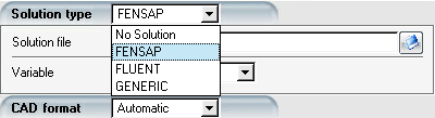
Select the input flow solution file with the browse  button. The flow solution type can be set to:
No solution: This option should be selected when only mesh smoothing is performed by OptiGrid. No solution files are required in this case.
FENSAP: FENSAP-ICE file format described in FENSAP-ICE File Formats.
FLUENT: In this case, the .dat(.h5) file should be loaded.
Note: The base filename for both .cas(.h5) (grid) and .dat(.h5) (solution) files must be the same directory.
GENERIC: FENSAP-ICE simplified format for mesh adaptation, described in FENSAP-ICE File Formats
Important: The solution file format should be the same as the mesh file format.
In this section you will set up and assign flow variables for error estimation within OptiGrid.
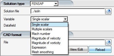
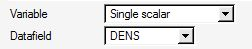
Variable sets the flow variable that is used to compute the error estimate:
Single scalar allows selecting one variable from the input solution file, all listed under Datafield. The list of variables can be modified in the Advanced menu.
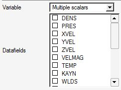
Multiple scalars option allows you to select more than one variable from the solution file. For this option, OptiGrid combines the contribution of all selected variables in error approximation. The list of variables in the solution file is provided as a list of check boxes.
The Mach number is computed by OptiGrid from the input flow solution as:

where  is the gas constant set to 1.4.
The Magnitude of velocity is computed by OptiGrid from the input flow solution as:

The Magnitude of vorticity is computed by OptiGrid from the input flow solution as:

If Expression is selected, OptiGrid constructs the scalar to be used for error estimate based on the expression supplied by you.
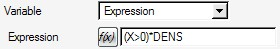
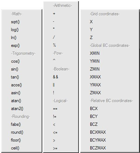
The expression can be a single field or a function of any of the flow variables present in the input solution file. Each of them should be referred to using its corresponding solver label in the solution file. The equation should be built using the provided variables, functions and operators:
Finally, select Mesh smoothing for grid smoothing only (no input solution provided).
Click the Advanced toolbar to specify the label of each input flow variable.
Specify opens a new window:
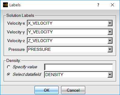
to create links between labels of the flow variables in the input solution file and OptiGrid’s standard names, in order to ensure full compatibility between the flow solver and OptiGrid.
Note: If the flow is incompressible and the density field is not stored in the solution file, a numeric value can be entered. In this way, the Mach number and y+ will be properly defined.
The flow variable used to compute the error should be chosen so as to best capture the desired, determining or dominant flow characteristics. The following guidelines help in selecting the appropriate flow variable:
For a subsonic Euler flow (without shocks), almost any sensible variable should work.
For a transonic or supersonic Euler flow (with shocks), the pressure is a good adaptation variable since it experiences a jump across each shock. The Mach number and density may also be used advantageously, because they can detect both shocks and contact discontinuities.
For subsonic Navier-Stokes solutions (without shocks), the Mach number can be used as the adaptation variable to capture the boundary layer, since the velocity gradient is strong normal to a wall. Using pressure as the adaptation variable is not recommended, since the pressure gradient is very weak across a boundary layer. However, to adapt for both the Mach number and the pressure, you must either use the Multiple scalars adaptation or define an expression of these variables.
For transonic Navier-Stokes solutions (with shocks), no ideal choice for the adaptation variable is obvious, as the Mach number is often not sensitive enough to capture shocks properly, giving too much emphasis to boundary layers. In this case it is suggested to use a combination of the Mach number and pressure using the Multiple scalars option or by defining a custom expression of these variables.
For the solutions with multiple separation zones, it is suggested to choose the Multiple scalars adaptation and then select all velocity components in order to capture separation lines accurately.
Enter the name and location of the geometry filename to be created by OptiGrid. You can also load a previously saved CAD file using the browse icon.
Click to automatically create a suitable CAD for the input mesh. This operation may take a few moments depending on the size of the grid.
For more advanced CAD operations, click . Detailed guidelines on how to use the CAD reconstruction tool are presented in OptiGrid - CAD Reconstruction.