


Below are examples of OptiGrid's theoretical background.
In order to adapt a grid to minimize the error throughout the computational domain, OptiGrid first needs to estimate the difference or error, e(x), between the exact solution g(x) and the numerical solution gh(x) of a given flow problem on a grid of size of O(h):

Of course, for most problems, except those with an exact solution, the error can only be estimated, as g(x) is generally unknown.
The global error e(x) has various sources:
Error resulting from the discretization of a continuum over a finite grid.
Grid-related errors, such as inappropriate grid distribution and misaligned grids.
Geometric approximations of solid boundaries.
Addition of stability and convergence enhancers, such as artificial viscosity, damping, smoothing and upwinding.
Incomplete convergence of the flow solver should it slow down or stall.
Computer round-off error.
A grid adapted by OptiGrid will minimize error sources 1 to 3, as new grid points will be placed or displaced, automatically, where needed to accurately capture the flow characteristics. For error sources 4 and 5, experience indicates that the flow solver usually requires less and less artificial viscosity as the grid gets optimized and, in addition, that convergence of the flow solver is improved. Round-off error is intrinsic to numerical calculations and is unaffected by OptiGrid.
OptiGrid is based on minimizing the difference between the PDE and its discretized form. Using a 1D Taylor expansion of both the exact (PDE) and numerical solutions (discretized), the truncation error can be estimated within an element, in 1D, to be:

where h is the element size and x is a local coordinate within the element (0,h). The error estimate over one element is computed as the maximum of e(x):

This indicates that the error is a direct function of the second derivative of the solution and not, as is used by many other mesh adaptation tools, a function of the gradients (first derivatives). This estimator is therefore a truer representation of the problem error.
The truncation error, derived for the 1D case, can be extended to 3D by considering the coordinates of each edge of the mesh, or

where  is the edge length and
  is the tangential direction of that edge. The second derivatives
of the numerical solution are computed along the direction
is the tangential direction of that edge. The second derivatives
of the numerical solution are computed along the direction  of an edge from

where

This error estimate is edge-based and the derived error estimate can therefore be computed for any element type (hexahedral, tetrahedral, prismatic, or pyramidal).
Furthermore, information about the error direction can be derived from the eigenvectors R of the Hessian matrix H, allowing anisotropic adaptation. In a shock, for example, cells will automatically be stretched by OptiGrid along the discontinuity direction, therefore requiring fewer grid points to accurately capture the shock than if isotropic adaptation was performed.
Several adaptation strategies are implemented in OptiGrid. These are categorized as follows:
Moving Nodes:
Equidistribute the error throughout the domain by moving the position of the grid points.
Refinement:
Reduce the error throughout the domain by adding new grid points where the error is higher than a target error threshold.
Coarsening:
Equidistribute the error throughout the domain by removing grid points where the error is lower than the target error threshold.
Edge Swapping:
Reconnect edges to optimize their orientation and to better align the grid to unidirectional flow features.
The best strategy is a combination of all four operations to minimize and make the error uniform everywhere, while maintaining an acceptable number of grid points (memory requirement). Node movement is the only continuous operation and it may be viewed as the driving force of mesh adaptation. Refinement, coarsening, and edge swapping are binary (yes/no) operations that complement the action of node movement and should be viewed as a way to accelerate convergence to an optimum grid.
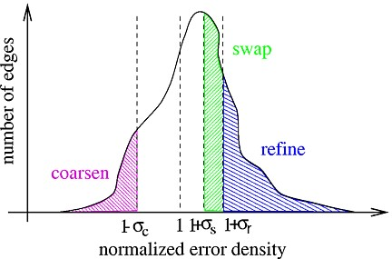
The next figure shows a typical distribution of the error density on the edges, normalized by the target error. The threshold levels for coarsening, swapping and refinement are set at (1-σc), (1+σs) and (1+σr), respectively.
In the node movement strategy, all edges connected to a given node xj are
viewed as a network of springs, with stiffness constants  proportional to the edge-based error, or

where  is the n node connected to node
  . The ideal position of node
  is then computed from a nonlinear energy minimization
problem:
is then computed from a nonlinear energy minimization
problem:

where

This equation is nonlinear and therefore, its solution is based on the iterative algorithm

which starts from an initial guess  and converges gradually to the location of equilibrium
  . The input parameter ω is a relaxation factor.
Note: The movement of one grid point modifies all the surrounding elements. For this reason, the node movement strategy should be repeated several times throughout the domain.
The mesh is refined if the error estimate on a given edge exceeds the target error by more than σr. In this case, a new node is introduced in the middle of the edge, and the connectivity of the nodes is updated accordingly. On boundary curves and surfaces, the new or collapsed node is projected back onto the CAD description of the boundary of the computational domain. Conversely, the mesh is coarsened if the error estimate on a given edge is below the coarsening threshold (1-σc). In that case, the edge is simply deleted and its two end points are collapsed, or merged, into a single point.
The edge swapping algorithm implemented in OptiGrid swaps the edges that connect a set of nodes. The optimal configuration is selected such that the error along the edges is minimized. A minimum aspect ratio in the Euclidean space must also be respected. Swapping is applicable to tetrahedral elements and to columns of prismatic elements. It is not supported for hexas and pyramids.
The role of swapping is to accelerate the alignment of edges with one-directional flow features such as shocks and boundary layers.
Tip: Swapping an edge modifies the surrounding elements. For that reason, the edge swapping strategy should be repeated several times throughout the domain.
OptiGrid adapts the grid in the following sequence:
Node movement is performed on boundaries to smooth out the grid on surfaces. This may be repeated several times, based on the user input.
Edge refinement and swapping on boundaries are performed according to a user-specified curvature criterion so as to better represent regions of high curvature.
Node movement is performed in the entire computational domain, including boundaries.
Edge refinement and coarsening are performed simultaneously in the entire domain, including boundaries.
Edge swapping is performed in the entire computational domain, including boundaries, in order to optimize the shape of elements. This is repeated several times based on the user input.
Node movement is performed in the entire computational domain, including boundaries, in order to smooth the adapted mesh (repeated several times based on the user input).
Note: Sequence 1 to 6 is referred to as one main iteration. Many main iterations can be performed by OptiGrid, based on the user’s input. If the initial grid is well suited to the flow, the mesh adaptation may require no more than 3 main iterations. If the initial grid is uniform or very coarse, the mesh adaptation may require up to 15 main iterations.