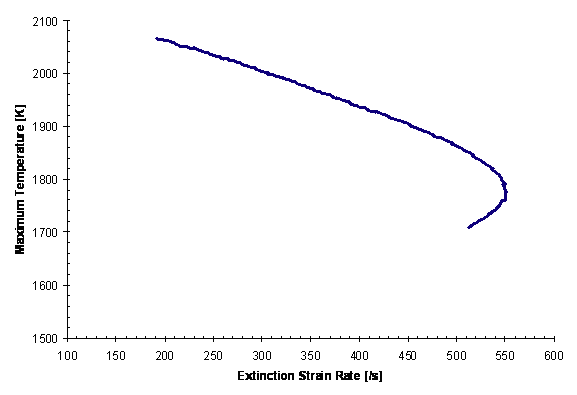
The Flame Extinction Simulator solves the same set of equations for a 1-D strained flame as the Opposed-flow Flame Simulator, as described in Axisymmetric and Planar Diffusion . However, this model is used to determine the extinction strain rate for the non-premixed or premixed flame conditions, through an iterative series of opposed-flow flame simulations. As flame strain rate is varied, the Flame-Extinction Simulator will predict an S-curve response for the flame temperature as a function of strain rate. The lower and upper branches of the temperature vs. strain-rate S-curve represent weak and strong solutions, respectively, while the middle branch represents unstable solutions. The lower and upper turning points are interpreted as the ignition and extinction points, respectively.

Figure 14.3: Flame response curve showing extinction (turning) for premixed stoichiometric methane-air flame. The inlet temperature is 296 K and ambient pressure is 1 atm. The calculated extinction strain rate is 550 /s.

Since the Jacobian matrix is singular at the turning points, a special technique called arc-length continuation [109] is used to compute the solutions through the turning points. In theory, one can calculate the solutions up to the turning point using successive continuations on velocity. Such a technique requires smaller and smaller changes in the velocity, accompanied by more computational difficulty to get a solution, as the extinction point is approached.

As described in Axisymmetric and Planar Diffusion , the Opposed-flow Flame Simulator solves for the variables T, F, G, H, and Yk. For the purpose of this discussion, while T is the temperature and Y _k is the species mass fraction of the k th species, F and G can be considered to represent the x and y velocities, respectively. H is the eigenvalue of the problem and represents the pressure curvature. This system of equations constitutes a two-point boundary value problem. The governing equations for T, G, and Y _k are second-order and hence require two (boundary) conditions. For the continuation analysis, the F and H equations are relevant and these are re-written here:

(14–21)

(14–22)

As two first-order differential equations, these two equations require two boundary conditions. Table 14.2: Summary of Boundary Conditions in the Opposed-flow Flame simulator shows a summary of the equations and associated boundary conditions used in the Opposed-Flow Flame Simulator.

As shown in Table 14.2: Summary of Boundary Conditions in the Opposed-flow Flame simulator , the Opposed-flow Flame Simulator uses the oxidizer inlet velocity as the boundary condition for the eigenvalue equation. Thus, effectively, information about F propagates from fuel to oxidizer inlet locations while "shooting" for the correct value at the oxidizer side. The corrective measure for the shooting is supplied by the H value propagating from oxidizer to fuel locations.

In principle, by swapping the roles of the response and control variables, it is possible to calculate all points along the full response curve for flame-extinction calculations. The Flame-Extinction Simulator uses a flame-controlling continuation as described in Takeno et al. [110]. Instead of performing continuations with the velocity from either nozzle, an additional constraint, in this case a fixed temperature at a particular grid point, is specified. This additional constraint means one boundary condition must be relaxed. The natural choice, in this case, would be the oxidizer velocity (U _o) or fuel velocity (U _f), such that the oxidizer (or fuel) velocity is obtained as a part of the solution. In theory, any number of such internal constraints can be specified on any solution variable: temperature, species mass fraction, etc. Depending upon the number, M, of constraints specified, the flame-controlling technique can be termed as M -point controlling.

It may be difficult or in some cases even impossible to go though the extinction point with one-point control. This is the case if the response variable of the continuation problem itself shows a turning-point behavior. In the case of the Flame-Extinction Simulator, the response variable is the oxidizer velocity or the pressure eigenvalue. Although one-point continuation is adequate for most of the cases, the Flame-Extinction Simulator can perform both one-point and two-point control. In the former case, temperature at a point on the fuel side is specified while in the latter temperature is specified at one point on both fuel and oxidizer sides.