


For the Opposed-flow Flame model, a steady-state solution is computed for either
axisymmetric or planar diffusion flames between two opposing nozzles. The opposed-flow
geometry makes an attractive experimental configuration, because the flames are flat,
allowing for detailed study of the flame chemistry and structure. The two or
three-dimensional flow is reduced mathematically to one dimension by assuming that the
 - or radial velocity varies linearly in the
  - or radial direction, which leads to a simplification in which the
fluid properties are functions of the axial distance only. The one-dimensional model
then predicts the species, temperature, and velocity profiles in the core flow between
the nozzles (neglecting edge effects). Both premixed and non-premixed flames can be
simulated.
- or radial direction, which leads to a simplification in which the
fluid properties are functions of the axial distance only. The one-dimensional model
then predicts the species, temperature, and velocity profiles in the core flow between
the nozzles (neglecting edge effects). Both premixed and non-premixed flames can be
simulated.
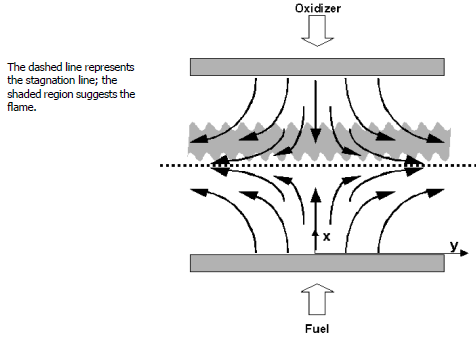
The axisymmetric geometry consists of two concentric, circular nozzles directed towards each other, as in Figure 14.1: Geometry of the axisymmetric opposed-flow diffusion flame . This configuration produces an axisymmetric flow field with a stagnation plane between the nozzles. The planar geometry consists of two concentric linear nozzles directed towards each other as shown in Figure 14.2: Geometry of the planar opposed-flow diffusion flame . This configuration produces a 2-D planar flow field with a stagnation line between the two nozzles. The location of the stagnation plane (line) depends on the momentum balance of the two streams. When the streams are premixed, two premixed flames exist, one on either side of the stagnation plane. When one stream contains fuel and the other oxidizer, a diffusion flame is established. Since most fuels require more air than fuel by mass, the diffusion flame usually sits on the oxidizer side of the stagnation plane; fuel diffuses through the stagnation plane to establish the flame in a stoichiometric mixture.
Our Opposed-flow Flame Simulator is derived from a model that was originally developed by Kee, et al. [104] for premixed opposed-flow flames. The reduction of the three-dimensional stagnation flow is based upon similarity solutions advanced for incompressible flows by von Karman, [105] which are more easily available in Schlichting [106]. The use of the similarity transformation is described in more detail in Stagnation-Flow and Rotating-Disk CVD . Note that the Ansys Chemkin impinging and stagnation-flow models are based on a finite domain, where the user specifies the nozzle separation. For this approach, an eigenvalue must be included in the solution of the equations and the strain rate varies, such that a characteristic strain rate must be determined from the velocity profile. Following the analysis of Evans and Grief, [107] Kee, et al. [104] showed that this formulation allowed more accurate predictions of the extinction limits for premixed flames than other approaches.
The geometry and axes for the axisymmetric and planar configurations are sketched in
Figure 14.1: Geometry of the axisymmetric opposed-flow diffusion flame
and Figure 14.2: Geometry of the planar opposed-flow diffusion flame
, respectively. In the
following equations,  represents either the radial direction
  for the axisymmetric case, or the perpendicular direction
 for the planar case. The coordinate parameter
  allows us to present one set of equations for both cases, with
 for the 3-D axisymmetric flow and
  for the 2-D planar case. A more detailed derivation of the governing
equations for the opposed-flow geometry is provided by Kee, et al.[104]
for the 2-D planar case. A more detailed derivation of the governing
equations for the opposed-flow geometry is provided by Kee, et al.[104]
At steady-state, conservation of mass in cylindrical or planar coordinates is
 | (14–1) |
where  and
and  are the axial and radial (or cross-flow) velocity components, and
 is the mass density.

Following von Karman, [105]
who recognized that
 and other variables should be functions of
  only, we define
for which the continuity Equation 14–1 reduces to
 | (14–2) |
for the axial velocity  . Since
  and
and  are functions of
  only, so are
  ,
,  ,
,  and
and  .
.
The perpendicular momentum equation is satisfied by the eigenvalue
 | (14–3) |
The perpendicular momentum equation is
 | (14–4) |
Energy and species conservation are
 | (14–5) |
where  is the heat loss due to gas and particle radiation which is described
in Gas and Particulate Thermal Radiation Model for Flames
.
is the heat loss due to gas and particle radiation which is described
in Gas and Particulate Thermal Radiation Model for Flames
.
 | (14–6) |
where the diffusion velocities are given by either the multicomponent formulation
 | (14–7) |
or the mixture-averaged formulation
 | (14–8) |
and  ,
,  ,
,  and
and  are the multicomponent, mixture-averaged, binary, and thermal
diffusion coefficients, respectively.
are the multicomponent, mixture-averaged, binary, and thermal
diffusion coefficients, respectively.
The boundary conditions for the fuel ( ) and oxidizer (
 ) streams at the nozzles are
 | (14–9) |
Note that the inflow boundary condition (Equation 14–9
) specifies the total mass
flux, including diffusion and convection, rather than the fixing species mass fraction
 . If gradients exist at the boundary, these conditions allow diffusion
into the nozzle.
. If gradients exist at the boundary, these conditions allow diffusion
into the nozzle.
The differential Equation 14–2
through Equation 14–6
and boundary conditions
Equation 14–9
form a boundary value
problem for the dependent variables ( ,
,  ,
,  ,
,  ,
,  ). The Gas-phase Kinetics Subroutine
Library provides the reaction rates and thermodynamic properties, while the
Transport package evaluates the transport properties
for these equations.
). The Gas-phase Kinetics Subroutine
Library provides the reaction rates and thermodynamic properties, while the
Transport package evaluates the transport properties
for these equations.