


Kazakov and Frenklach [149] developed an aggregation model to work in conjunction with the moments method to obtain the distribution of the number of primary particles forming aggregates. While the particle aggregation model of Kazakov and Frenklach allows the prediction of both the average number of primary particles in the aggregates and its variation (standard deviation), this aggregation model does have drawbacks. To obtain the moments of the distribution of the number of primary particles in aggregates, Kazakov and Frenklach’s model needs to solve at least two additional moments equations, which are known to be difficult to converge. The additional hard computational work does not provide added benefits, as their aggregation model does not consider the correlation between the size of primary particles and the size of (or the number of primary particles in) the aggregates. The other major issue of the Kazakov-Frenklach aggregation model is the omission of the particle sintering effect [151]. The particle sintering model addresses the competition between coalescence and aggregation, when the particles are brought in contact, and determines the outcome of the collision: a larger primary particle or an aggregate formed by the colliding particles. Without a sintering model, the Kazakov-Frenklach aggregation model would treat all collisions as either strictly coalescent or strictly aggregate.
Building on the method of moments of Frenklach and Harris [152], Mueller et al. implemented a soot aggregation model based on the volume-surface correlation of aggregates. Rather than tracking the moments of aggregate size distribution and moments of primary particle distribution among the aggregates, the joint volume-surface aggregate model solves moments of volume and surface area of aggregates. This aggregate model does allow the inclusion of the particle sintering effect. However, because only aggregate volume and surface area are utilized by this model, it is not straightforward to incorporate physical parameters that actually govern the particle sintering process. Average aggregate properties such as collision diameter and number of primary particles can be computed from aggregate volume and surface area according to the fractal geometry relationship. This aggregate model requires at least 5 moments to properly track the joint volume-surface moments and the authors recommend solving 6 moments.
The relatively simple particle aggregation model implemented with the Particle Tracking feature is also compatible with the moments method. However, it attempts to amend problems associated with the aggregation models of Kazakov and of Mueller, while still providing aggregate properties such as average number of primary particles and average surface area. The aggregation model addresses those disadvantages of other moments-based aggregation models by the inclusion of a particle surface-area equation. By finding connections between average aggregate surface area and the fractal geometry relationship, this aggregation model solves only one additional equation and does not require solution of additional moments. A particle sintering model is incorporated into the surface area equation so that the particle-sintering effect, yielding aggregates in various degrees of fusion, is reflected by the change in particle surface area after collision. The particle-sintering model determines the extent of fusion by comparing the time scales of particle collision and particle fusion.
The aggregation model is capable of providing average aggregate properties such as number of primary particles in an aggregate, aggregate collision diameter, and diameter of the primary particle in addition to overall aerosol characteristics (number density, surface area density, and volume fraction). The only information available from the other aggregation models but not from this model is the variance of the number of primary particles among aggregates.
The moments method implemented in the Particle Tracking feature models the
aggregation process by keeping track of the particle surface area. Thus, the total particle
surface area (per volume) is solved by a surface area equation, which assumes that particle
area is modified by aggregation, as well as by nucleation, coagulation and mass
growth/reduction due to surface reactions. This model is designed to be easily solved
alongside the particle size moments. Because both mass growth and coagulation effects are
included in the moment equations, the surface area equation needs to consider only the
difference in area growth when the collision does not result in coagulation (or fusion) but
instead by aggregation. The transport equation for total particle surface area per volume
 is given as
 | (19–136) |
 is the portion of particle diffusion coefficient that is independent of
particle size and is given as
is the portion of particle diffusion coefficient that is independent of
particle size and is given as
 | (19–137) |
 [cm2/cm3-sec] is the total particle surface area production rate and
consists of contributions from three sources: nucleation, surface growth, and the combined
effect of coagulation and aggregation, that is,
[cm2/cm3-sec] is the total particle surface area production rate and
consists of contributions from three sources: nucleation, surface growth, and the combined
effect of coagulation and aggregation, that is,
 | (19–138) |
If the nucleation rate is r nuc [mole/cm3-sec] and the inception class of the particle is j nuc, the surface area production rate due to nucleation can be calculated as
 | (19–139) |
or, in general form, as
 | (19–140) |
The surface area production due to the particle mass growth surface reactions can be obtained from the surface growth contribution to the two-third moment:
 | (19–141) |
where  is the contribution of the is -th surface reaction to
the production of the two-third size moment.
is the contribution of the is -th surface reaction to
the production of the two-third size moment.
When only particle aggregation is considered, the particle surface area production rate (or actually destruction rate) is interpolated from the production rates of the whole moments:
 | (19–142) |
On the other hand, in the absence of particle coagulation, the pure aggregation process yields no surface area change if the contact surface areas between primary particles in the aggregate are assumed to be negligible; that is,
 | (19–143) |
If both particle coagulation and aggregation are considered, the actual
surface area production rate due to these two processes should lay between  and
and  . To determine the weight between contributions from these two processes, a
measure of their relative importance is considered. Since the final particle structure after
collision depends on two characteristic time scales: the characteristic collision time
. To determine the weight between contributions from these two processes, a
measure of their relative importance is considered. Since the final particle structure after
collision depends on two characteristic time scales: the characteristic collision time
 and the characteristic fusion time
  , the ratio of these two characteristic time scales serve as the weighting
parameter.
, the ratio of these two characteristic time scales serve as the weighting
parameter.
 | (19–144) |
M 0 is the zero-th particle size moment and G 0 is the coalescent coagulation contribution to the production (destruction) of the zero-th size moment.
Now we define a parameter  to represent the relative importance of coalescence over aggregation
as
to represent the relative importance of coalescence over aggregation
as
 | (19–145) |
And the surface area production rate due to the combined effect of particle coagulation and aggregation can be written as
 | (19–146) |
By combining Equations Equation 19–130 and Equation 19–144 into Equation 19–146 , the particle surface production rate from coagulation and aggregation can be expressed as
 | (19–147) |
The average primary particle diameter  in Equations Equation 19–126
and Equation 19–130
is replaced by
in Equations Equation 19–126
and Equation 19–130
is replaced by  in Equation 19–147
, because collisions can occur
between primary particles as well as aggregates.
in Equation 19–147
, because collisions can occur
between primary particles as well as aggregates.  is the diameter of the sphere whose volume is the same as the average
volume of the aggregates and is given as
is the diameter of the sphere whose volume is the same as the average
volume of the aggregates and is given as
 | (19–148) |
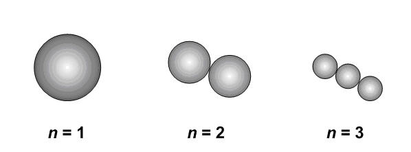
For use of the aggregation model, the concept of "particle class" in the Particle Tracking module is extended from being "the number of bulk species in a primary particle" to being "the total number of bulk species in primary particles forming the aggregate". Let n denote the number of primary particles in an aggregate. A class j "particle" without aggregation always indicates a spherical primary particle consisting of j bulk species; that is, n is always equal to 1. The same j -class "particle" could have many different configurations when aggregation is present, depending on the value of n, as shown schematically in Figure 19.16: Depending on the value of n, an aggregate of given class can have various configurations. .
Figure 19.16: Depending on the value of n, an aggregate of given class can have various configurations.
The average number of primary particles in aggregates,  , is obtained from the total particle surface area,
  , which is solved by Equation 19–136
. Assuming the primary
particles in an aggregate are spherical and are connected with each other at one point;
then the contact surface area is almost zero. The total surface area of an average
aggregate is computed by
, which is solved by Equation 19–136
. Assuming the primary
particles in an aggregate are spherical and are connected with each other at one point;
then the contact surface area is almost zero. The total surface area of an average
aggregate is computed by
 | (19–149) |
Alternatively, the same average aggregate surface area can be obtained from the total particle surface area as
 | (19–150) |
where M 0 is the zero-th moment of the particle size
distribution which represents the particle number density of the aerosol population. By
combining Equations Equation 19–149
andEquation 19–150
, an equation for  is derived to be
 | (19–151) |
Since the average class of primary particle in the aggregate
 is derived from the size moments as
 | (19–152) |
the average primary particle diameter in the aggregate,  , is expressed in terms of the size distribution moments [153]:
 | (19–153) |
Therefore, the average number of primary particles in aggregates is obtained by substituting Equation 19–153 into Equation 19–151 :
 | (19–154) |
Note that  should have a value between 1 and M
1/M 0. The collision diameter of the aggregate is then computed
by
[149]
:
should have a value between 1 and M
1/M 0. The collision diameter of the aggregate is then computed
by
[149]
:
 | (19–155) |
where D f is the fractal dimension of the aggregate. Typically, D f is about 1.8 for soot aggregates in flame environments[149] .
For a spherical particle of class j, its collision diameter can be easily calculated as[153] :
 | (19–156) |
The collision diameter of a non-spherical aggregate of the same class can be obtained from Equation 19–155 , with the help of the singe-size primary particle assumption, as
 | (19–157) |
By comparing Equations Equation 19–156
and Equation 19–157
, the collision frequency formulation
can be systematically modified by replacing all one-third moments with the  -th moment and by scaling the unit diameter
  by a factor of
  .
.
Accordingly, for collision frequency in the free-molecular regime, the collision frequency coefficient becomes
 | (19–158) |
and the function  becomes
 | (19–159) |
where
 .
.
The production rate of the r -th moment due to free-molecular aggregation can be expressed as
 | (19–160) |
The free-molecular coagulation rates given by Equation 19–160
are in general valid for
 . That is, highly non-spherical particles can sometimes pass through each
other without collision because of the large empty space within the collision diameter.
However, this deficiency can be amended by using a smaller collision efficiency β.
. That is, highly non-spherical particles can sometimes pass through each
other without collision because of the large empty space within the collision diameter.
However, this deficiency can be amended by using a smaller collision efficiency β.
Similarly, for collisions in the continuum regime, the production rate of the r -th due to aggregation can be rewritten as:
 | (19–161) |