


This tutorial simulates a static mixer consisting of two inlet pipes delivering water into a mixing vessel; the water exits through an outlet pipe. A general workflow is established for analyzing the flow of fluid into and out of a mixer using Ansys Workbench.
This tutorial includes:
In this tutorial you will learn about:
Using Ansys Workbench to set up a project.
Using Quick Setup mode in CFX-Pre to set up a problem.
Using Ansys CFX-Solver Manager to obtain a solution.
Modifying the outline plot in CFD-Post.
Using streamlines in CFD-Post to trace the flow field from a point.
Viewing temperature using colored planes and contours in CFD-Post.
Creating an animation and saving it as a movie file.
|
Component |
Feature |
Details |
|---|---|---|
|
CFX-Pre |
User Mode |
Quick Setup mode |
|
Analysis Type |
Steady State | |
|
Fluid Type |
General Fluid | |
|
Domain Type |
Single Domain | |
|
Turbulence Model |
k-Epsilon | |
|
Heat Transfer |
Thermal Energy | |
|
Boundary Conditions |
Inlet (Subsonic) | |
|
Outlet (Subsonic) | ||
|
Wall: No-Slip | ||
|
Wall: Adiabatic | ||
|
Timestep |
Physical Time Scale | |
|
CFD-Post |
Animation |
Keyframe |
|
Plots |
Contour | |
|
Outline Plot (Wireframe) | ||
|
Point | ||
|
Slice Plane | ||
|
Streamline |
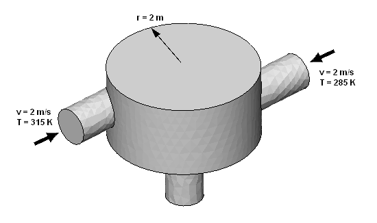
This tutorial simulates a static mixer consisting of two inlet pipes delivering water into a mixing vessel; the water exits through an outlet pipe. A general workflow is established for analyzing the flow of fluid into and out of a mixer.
Water enters through both pipes at the same rate but at different temperatures. The first entry is at a rate of 2 m/s and a temperature of 315 K and the second entry is at a rate of 2 m/s at a temperature of 285 K. The radius of the mixer is 2 m.
Your goal in this tutorial is to understand how to use CFX in Workbench to determine the speed and temperature of the water when it exits the static mixer.
If this is the first tutorial you are working with, it is important to review the following topics before beginning:
Create a working directory.
Ansys CFX uses a working directory as the default location for loading and saving files for a particular session or project.
Download the
static_mixer_workbench.zipfile here .Unzip
static_mixer_workbench.zipto your working directory.Ensure that the following tutorial input file is in your working directory:
StaticMixerMesh.gtm
Start Ansys Workbench.
To launch Ansys Workbench on Windows, click the Start menu, then select All Programs > Ansys 2024 R2 > Workbench 2024 R2.
To launch Ansys Workbench on Linux, open a command line interface, type the path to
runwb2(for example,~/ansys_inc/v242/Framework/bin/Linux64/runwb2), then press Enter.
From the main menu, select File > Save As.
In the Save As dialog box, browse to the working directory and set File name to
StaticMixer.Click .
Because you are starting with an existing mesh, you can immediately use CFX-Pre to define the simulation. To launch CFX-Pre:
In the Toolbox pane, open Component Systems and double-click CFX.
A CFX system opens in the Project Schematic.
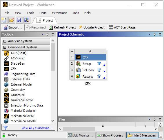
Note: You use a CFX component system because you are starting with a mesh. If you wanted to create the geometry and mesh, you would start with a Fluid Flow (CFX) analysis system.
Right-click the blue CFX cell (A1) and select Rename.
Change the name of the system to
Static Mixer. Finish by pressing Enter or by clicking outside the cell.In Ansys Workbench, enable View > Files and View > Progress so that you can see the files that are written and the time remaining to complete operations.
In the Workbench Project Schematic, double-click the Setup cell of the CFX component system.
CFX-Pre opens.
Optionally, change the background color of the viewer in CFX-Pre for improved viewing:
Select Edit > Options.
The Options dialog box appears.
Adjust the color settings under CFX-Pre > Graphics Style.
For example, you could set the Background > Color Type to Solid and the Color to white.
Click .
Before importing and working with the mesh, you need to create a simulation; in this example, you will use Quick Setup mode. Quick Setup mode provides a simple wizard-like interface for setting up simple cases. This is useful for getting familiar with the basic elements of a CFD problem setup.
In CFX-Pre, select Tools > Quick Setup Mode.
The Quick Setup Wizard opens, enabling you to define this single-phase simulation.
Under Working Fluid > Fluid select
Water.This is a fluid already defined in the library of materials as water at 25°C.
Under Mesh Data > Mesh File, click Browse
 .
.The Import Mesh dialog box appears.
Under Files of type, select
CFX Mesh (*gtm *cfx).From your working directory, select
StaticMixerMesh.gtm.Click Open.
The mesh loads, which enables you to apply physics.
Click Next.
You need to define the type of flow and the physical models to use in the fluid domain.
The flow is steady-state and you will specify the turbulence
and heat transfer. Turbulence is modeled using the  -
- turbulence
model and heat transfer using the thermal energy model. The
turbulence
model and heat transfer using the thermal energy model. The  -
- turbulence
model is a commonly used model and is suitable for a wide range of
applications. The thermal energy model neglects high speed energy
effects and is therefore suitable for low speed flow applications.
turbulence
model is a commonly used model and is suitable for a wide range of
applications. The thermal energy model neglects high speed energy
effects and is therefore suitable for low speed flow applications.
Under Model Data, note that the Reference Pressure is set to
1 [atm].All other pressure settings are relative to this reference pressure.
Set Heat Transfer to
Thermal Energy.Set Turbulence to
k-Epsilon.Click Next.
The CFD model requires the definition of conditions on the boundaries of the domain.
Delete
InletandOutletfrom the list by right-clicking each and selecting Delete Boundary.Right-click in the blank area where
InletandOutletwere listed, then select Add Boundary.Set Name to
in1.Click .
The boundary is created and, when selected, properties related to the boundary are displayed.
Once boundaries are created, you need to create associated data. Based on Figure 3.1: Static Mixer with 2 Inlet Pipes and 1 Outlet Pipe, you will define the velocity and temperature for the first inlet.
Set in1 > Boundary Type to
Inlet.Set Location to
in1.Set the Flow Specification > Option to
Normal Speedand set Normal Speed to:2 [m s^-1]Set the Temperature Specification > Static Temperature to
315 [K](note the units).
Based on Figure 3.1: Static Mixer with 2 Inlet Pipes and 1 Outlet Pipe, you know the second inlet boundary condition consists of a velocity of 2 m/s and a temperature of 285 K at one of the side inlets. You will define that now.
Under the Boundary Definition panel, right-click in the selector area and select Add Boundary.
Create a new boundary named
in2with these settings:Setting
Value
in2
> Boundary Type
Inlet
in2
> Location
in2
Flow Specification
> Option
Normal Speed
Flow Specification
> Normal Speed
2 [m s^-1]
Temperature Specification
> Static Temperature
285 [K]
Now that the second inlet boundary has been created, the same concepts can be applied to building the outlet boundary.
Create a new boundary named
outwith these settings:Setting
Value
out
> Boundary Type
Outlet
out
> Location
out
Flow Specification
> Option
Average Static Pressure
Flow Specification
> Relative Pressure
0 [Pa]
Click Next.
There are no further boundary conditions that need to be set. All 2D exterior regions that have not been assigned to a boundary condition are automatically assigned to the default boundary condition.
Set Operation to
Enter General Mode.Click Finish.
The three boundary conditions are displayed in the viewer as sets of arrows at the boundary surfaces. Inlet boundary arrows are directed into the domain. Outlet boundary arrows are directed out of the domain.
Now that the simulation is loaded, take a moment to explore how you can use the viewer toolbar to zoom in or out and to rotate the object in the viewer.
There are several icons available for controlling the level of zoom in the viewer.
Click Zoom Box

Click and drag a rectangular box over the geometry.
Release the mouse button to zoom in on the selection.
The geometry zoom changes to display the selection at a greater resolution.
Click Fit View
 to re-center and re-scale the geometry.
If you need to rotate an object or to view it from a new angle, you can use the viewer toolbar.
Click Rotate
 on the viewer toolbar.
Click and drag within the geometry repeatedly to test the rotation of the geometry.
The geometry rotates based on the direction of mouse movement and based on the initial mouse cursor shape, which changes depending on where the mouse cursor is in the viewer. If the mouse drag starts near a corner of the viewer window, the motion of the geometry will be constrained to rotation about a single axis, as indicated by the mouse cursor shape.

Right-click a blank area in the viewer and select Predefined Camera > View From -X.
Right-click a blank area in the viewer and select Predefined Camera > Isometric View (Z Up).
A clearer view of the mesh is displayed.
Solver Control parameters control aspects of the numerical solution generation process.
While an upwind advection scheme is less accurate than other advection schemes, it is also more robust. This advection scheme is suitable for obtaining an initial set of results, but in general should not be used to obtain final accurate results.
The time scale can be calculated automatically by the solver
or set manually. The Automatic option tends to
be conservative, leading to reliable, but often slow, convergence.
It is often possible to accelerate convergence by applying a time
scale factor or by choosing a manual value that is more aggressive
than the Automatic option. In this tutorial,
you will select a physical time scale, leading to convergence that
is twice as fast as the Automatic option.
In the CFX-Pre toolbar, click Solver Control
 .
.On the Basic Settings tab, set Advection Scheme > Option to
Upwind.Set Convergence Control > Fluid Timescale Control > Timescale Control to
Physical Timescaleand set the physical timescale value to2 [s].Click .
To obtain a solution, you need to launch the CFX-Solver Manager and subsequently use it to start the solver:
Double-click the Ansys Workbench Solution cell. The CFX-Solver Manager appears with the Define Run dialog box displayed.
The Define Run dialog box enables configuration of a run for processing by CFX-Solver. In this case, all of the information required to perform a new serial run (on a single processor) is entered automatically. You do not need to alter the information in the Define Run dialog box.
Optionally specify a local parallel run:
Set Run Mode to a parallel mode suitable for your configuration; for example,
Intel MPI Local Parallel.This is the recommended method for most applications.
If required, click Add Process
 to increase the maximum number of processes.
Ideally, the number of processes should not exceed the number of available processor cores. The number of processes used will be the number of partitions for the mesh.
More detailed information about setting up CFX to run in parallel is available in Flow Around a Blunt Body.
Click Start Run.
CFX-Solver launches and a split screen appears and displays the results of the run graphically and as text. The panes continue to build as CFX-Solver Manager operates.
One window shows the convergence history plots and the other displays text output from CFX-Solver. The text lists physical properties, boundary conditions, and various other parameters used or calculated in creating the model. All the text is written to the CFX-Solver Output file automatically (in this case,
StaticMixer_001.out).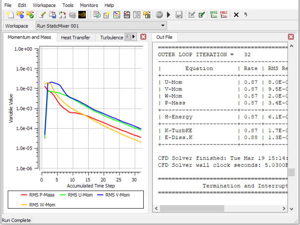
Note: Once the second iteration appears, data begins to plot. Plotting may take a long time depending on the amount of data to process. Let the process run.
When CFX-Solver is finished, a message is displayed and the final line in the CFX-Solver Output file (which you can see in the CFX-Solver Manager) is:
This run of the Ansys CFX Solver has finished.
Once CFX-Solver has finished, you can use CFD-Post to review the finished results:
In Ansys Workbench, right-click the Results cell and select Refresh.
When the refresh is complete, double-click the Results cell. CFD-Post appears.
When CFD-Post starts, the viewer and Outline workspace are displayed. Optionally, change the background color of the viewer for improved viewing:
In CFD-Post, select Edit > Options. The Options dialog box appears.
Adjust the color settings under CFD-Post > Viewer. For example, you could set the Background > Color Type to Solid and the Color to white.
Click .
The viewer displays an outline of the geometry and other graphic objects. You can use the mouse or the toolbar icons to manipulate the view, exactly as in CFX-Pre.
The tutorial follows this general workflow for viewing results in CFD-Post:
- 3.7.1. Setting the Edge Angle for a Wireframe Object
- 3.7.2. Creating a Point for the Origin of the Streamline
- 3.7.3. Creating a Streamline Originating from a Point
- 3.7.4. Rearranging the Point
- 3.7.5. Configuring a Default Legend
- 3.7.6. Creating a Slice Plane
- 3.7.7. Defining Slice Plane Geometry
- 3.7.8. Configuring Slice Plane Views
- 3.7.9. Rendering Slice Planes
- 3.7.10. Coloring the Slice Plane
- 3.7.11. Moving the Slice Plane
- 3.7.12. Adding Contours
- 3.7.13. Working with Animations
- 3.7.14. Closing the Applications
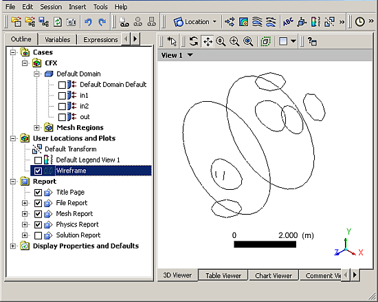
The outline of the geometry is called the wireframe or outline plot.
By default, CFD-Post displays only some of the surface mesh.
This sometimes means that when you first load your results file, the
geometry outline is not displayed clearly. You can control the amount
of the surface mesh shown by editing the Wireframe object listed in the Outline.
The check boxes next to each object name in the Outline tree view control the visibility of each object. Currently only
the Wireframe and Default Legend objects have visibility turned on.
The edge angle determines how much of the surface mesh is visible. If the angle between two adjacent faces is greater than the edge angle, then that edge is drawn. If the edge angle is set to 0°, the entire surface mesh is drawn. If the edge angle is large, then only the most significant corner edges of the geometry are drawn.
For this geometry, a setting of approximately 15° lets you view the model location without displaying an excessive amount of the surface mesh.
In this module you can also modify the zoom settings and view of the wireframe.
In the Outline, under
User
Locations and Plots
, double-clickWireframe.Right-click a blank area anywhere in the viewer, select Predefined Camera from the shortcut menu, and select Isometric View (Z up).
Tip: While it is not necessary to change the view to set the edge angle for the wireframe, doing so enables you to explore the practical uses of this feature.
In the Wireframe details view, under Definition, click in the Edge Angle box.
An embedded slider is displayed.
Type a value of
10 [degree].Click Apply to update the object with the new setting.
Notice that more surface mesh is displayed.

Drag the embedded slider to set the Edge Angle value to approximately
45 [degree].Click Apply to update the object with the new setting.
Less of the outline of the geometry is displayed.
Type a value of
15 [degree].Click Apply to update the object with the new setting.
A streamline is the path that a particle of zero mass would follow through the domain.
Select Insert > Location > Point from the main menu.
You can also use the toolbars to create a variety of objects. Later modules and tutorials will explore this further.
Click .
This accepts the default name.
Set Definition > Method to
XYZ.Under Point, enter the following coordinates:
-1, -1, 1.This is a point near the first inlet.
Click Apply.
The point appears as a symbol in the viewer as a crosshair symbol.
Where applicable, streamlines can trace the flow direction forwards (downstream) and/or backwards (upstream).
From the main menu, select Insert > Streamline.
Click .
Set Definition > Start From to
Point 1.Tip: To create streamlines originating from more than one location, click the Ellipsis
 icon to the right of the Start From box. This displays the Location Selector dialog
box, where you can use the Ctrl and Shift keys to pick multiple locators.
icon to the right of the Start From box. This displays the Location Selector dialog
box, where you can use the Ctrl and Shift keys to pick multiple locators.Click the Color tab.
Set Mode to
Variable.Set Variable to
Total Temperature.Set Range to
Local.Click Apply.
The streamline shows the path of a zero mass particle from
Point 1. The temperature is initially high near the hot inlet, but as the fluid mixes the temperature drops.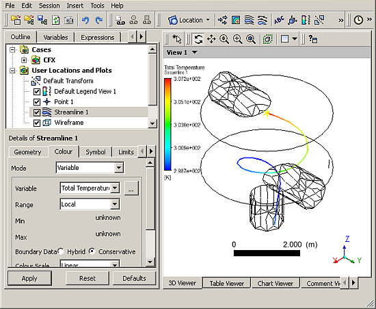
Once created, a point can be rearranged manually or by setting specific coordinates.
Tip: In this module, you may choose to display various views and
zooms from the Predefined Camera option in the
shortcut menu (such as Isometric View (Z up) or View From -X) and by using Zoom Box if you prefer to change the display.
In Outline, under
User Locations and Plotsdouble-clickPoint 1.Properties for the selected user location are displayed.
Under Point, set these coordinates:
-1, -2.9, 1.Click Apply.
The point is moved and the streamline redrawn.
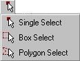
In the viewer toolbar, click Select
 and ensure that the adjacent toolbar icon is
set to Single Select
and ensure that the adjacent toolbar icon is
set to Single Select  .
.
While in select mode, you cannot use the left mouse button to re-orient the object in the viewer.
In the viewer, drag
Point 1(appears as a yellow addition sign) to a new location within the mixer.The point position is updated in the details view and the streamline is redrawn at the new location. The point moves normal in relation to the viewing direction.
Click Rotate
.Tip: You can also click in the viewer area, and press the space bar to toggle between Select and Viewing Mode. A way to pick objects from Viewing Mode is to hold down Ctrl + Shift while clicking on an object with the left mouse button.
Under Point, reset these coordinates:
-1, -1, 1.Click Apply.
The point appears at its original location.
Right-click a blank area in the viewer and select Predefined Camera > View From -X.
You can modify the appearance of the default legend.
The default legend appears whenever a plot is created that is colored by a variable. The streamline color is based on temperature; therefore, the legend shows the temperature range. The color pattern on the legend’s color bar is banded in accordance with the bands in the plot.
Note: If a user-specified range is used for the legend, one or more bands may represent values beyond the legend’s range. In this case, these band colors are extrapolated slightly past the range of colors shown in the legend.
The default legend displays values for the last eligible plot
that was opened in the details view. To maintain a legend definition
during a CFD-Post session, you can create a new legend by clicking Legend  .
.
Because there are many settings that can be customized for the legend, this module allows you the freedom to experiment with them. In the last steps you will set up a legend, based on the default legend, with a minor modification to the position.
Tip: When editing values, you can restore the values that were present when you began editing by clicking Reset. To restore the factory-default values, click Default.
Double-click
Default Legend View 1.The Definition tab of the default legend is displayed.
Configure the following setting(s):
Tab
Setting
Value
Definition
Title Mode
User Specified
Title
Streamline Temp.
Horizontal
(Selected)
Location
> Y Justification
Bottom
Click Apply.
The appearance and position of the legend changes based on the settings specified.
Modify various settings in Definition and click Apply after each change.
Select Appearance.
Modify a variety of settings in the Appearance and click Apply after each change.
Click Defaults.
Click Apply.
Under Outline, in
User
Locations and Plots
, clear the check boxes forPoint 1andStreamline 1.Since both are no longer visible, the associated legend no longer appears.
Defining a slice plane allows you to obtain a cross-section of the geometry.
In CFD-Post you often view results by coloring a graphic object. The graphic object could be an isosurface, a vector plot, or in this case, a plane. The object can be a fixed color or it can vary based on the value of a variable.
You already have some objects defined by default (listed in the Outline). You can view results on the boundaries of the static mixer by coloring each boundary object by a variable. To view results within the geometry (that is, on non-default locators), you will create new objects.
You can use the following methods to define a plane:
Three Points: creates a plane from three specified points.Point and Normal: defines a plane from one point on the plane and a normal vector to the plane.YZ Plane,ZX Plane, andXY Plane: similar toPoint and Normal, except that the normal is defined to be normal to the indicated plane.
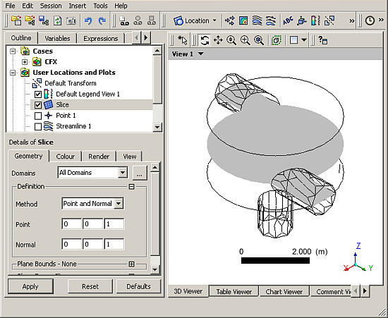
From the main menu, select Insert > Location > Plane or click Location > Plane.
In the Insert Plane window, type:
SliceClick .
The details view for the plane appears; the Geometry, Color, Render, and View tabs enable you to configure the characteristics of the plane.
You need to choose the vector normal to the plane. You want the plane to lie in the x-y plane, hence its normal vector points along the Z axis. You can specify any vector that points in the Z direction, but you will choose the most obvious (0,0,1).
On the Geometry tab, expand Definition.
Under Method select
Point and Normal.Under Point enter
0,0,1.Under Normal enter
0,0,1.Click Apply.
Sliceappears under User Locations and Plots. Rotate the view to see the plane.
Depending on the view of the geometry, various objects may not appear because they fall in a 2D space that cannot be seen.
Right-click a blank area in the viewer and select Predefined Camera > Isometric View (Z up).
The slice is now visible in the viewer.
Click Zoom Box
.Click and drag a rectangular selection over the geometry.
Release the mouse button to zoom in on the selection.
Click Rotate
.Click and drag the mouse pointer down slightly to rotate the geometry towards you.
Select Isometric View (Z up) as described earlier.
Render settings determine how the plane is drawn.
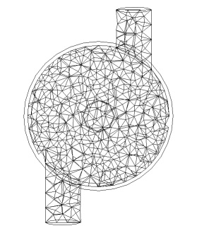
In the details view for Slice, select the Render tab.
Clear Show Faces.
Select Show Mesh Lines.
Under Show Mesh Lines change Color Mode to
User Specified.Click the current color in Line Color to change to a different color.
For a greater selection of colors, click the Ellipsis
icon to use the Color selector dialog box.Click Apply.
Click Zoom Box
.Zoom in on the geometry to view it in greater detail.
The line segments show where the slice plane intersects with mesh element faces. The end points of each line segment are located where the plane intersects mesh element edges.
Right-click a blank area in the viewer and select Predefined Camera > View From +Z.
The image shown below can be used for comparison with Flow in a Static Mixer (Refined Mesh) (in the section Creating a Slice Plane), where a refined mesh is used.
The Color panel is used to determine how the object faces are colored.
Configure the following setting(s) of
Slice:Tab
Setting
Value
Color
Mode
Variable [ a ]
Variable
Temperature
Render
Show Faces
(Selected)
Show Mesh Lines
(Cleared)
Click Apply.
Hot water (red) enters from one inlet and cold water (blue) from the other.
You can move the plane to different locations:
Right-click a blank area in the viewer and select Predefined Camera > Isometric View (Z up) from the shortcut menu.
Click the Geometry tab.
Review the settings in Definition under Point and under Normal.
Click Single Select
 .
.Click and drag the plane to a new location that intersects the domain.
As you drag the mouse, the viewer updates automatically. Note that Point updates with new settings.
Type in Point settings of
0,0,1.Click Apply.
Click Rotate
.Turn off the visibility for
Sliceby clearing the check box next toSlicein the Outline tree view.
Contours connect all points of equal value for a scalar variable
(for example, Temperature) and help to visualize
variable values and gradients. Colored bands fill the spaces between
contour lines. Each band is colored by the average color of its two
bounding contour lines (even if the latter are not displayed).
Right-click a blank area in the viewer and select Predefined Camera > Isometric View (Z up) from the shortcut menu.
Select Insert > Contour from the main menu or click Contour
 .
.The Insert Contour dialog box is displayed.
Set Name to
Slice Contour.Click .
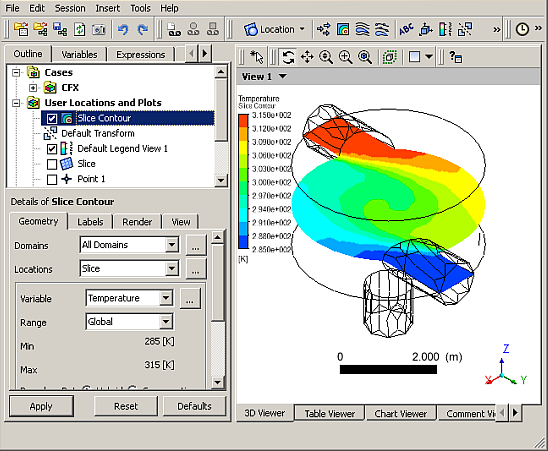
Configure the following setting(s):
Tab
Setting
Value
Geometry
Locations
Slice
Variable
Temperature
Render
Show Contour Lines
(Selected)
Click Apply.
Important: The colors of 3D graphics object faces are slightly altered when lighting is on. To view colors with highest accuracy, go to the Render tab and, under Show Faces, clear Lighting and click Apply.
The graphic element faces are visible, producing a contour plot as shown.
Note: Make sure that the visibility of Slice (in the Outline tree view) is turned off.
Animations build transitions between views for development of video files.
The tutorial follows this general workflow for creating a keyframe animation:
The Animation dialog box is used to define keyframes and to export to a video file.
Select Tools > Animation or click Animation
 .
.The Animation dialog box appears.
Set Type to Keyframe Animation.
Keyframes are required in order to produce a keyframe animation. You need to define the first viewer state, a second (and final) viewer state, and set the number of interpolated intermediate frames.
Right-click a blank area in the viewer and select Predefined Camera > Isometric View (Z up).
In the Outline, under
User
Locations and Plots
, turn off the visibility ofSlice Contourand turn on the visibility ofSlice.In the Animation dialog box, click New
 .
.A new keyframe named
KeyframeNo1is created. This represents the current image displayed in the viewer.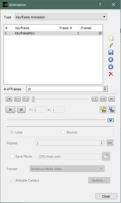
Define the second keyframe and the number of intermediate frames:
In the Outline, under
User
Locations and Plots
, double-clickSlice.On the Geometry tab, set Point coordinate values to
(0,0,-1.99).Click Apply.
The slice plane moves to the bottom of the mixer.
In the Animation dialog box, click New
.KeyframeNo2is created and represents the image displayed in the viewer.Select
KeyframeNo1so that you can set the number of frames to be interpolated between the two keyframes.Set # of Frames (located below the list of keyframes) to
20.This is the number of intermediate frames used when going from
KeyframeNo1toKeyframeNo2. This number is displayed in the Frames column forKeyframeNo1.Press Enter.
The Frame # column shows the frame in which each keyframe appears.
KeyframeNo1appears at frame 1 since it defines the start of the animation.KeyframeNo2is at frame 22 since you have 20 intermediate frames (frames 2 to 21) in betweenKeyframeNo1andKeyframeNo2.
More keyframes could be added, but this animation has only two keyframes (which is the minimum possible).
The controls previously grayed-out in the Animation dialog box are now available. The number of intermediate frames between keyframes is listed beside the keyframe having the lowest number of the pair. The number of frames listed beside the last keyframe is ignored.
Click To Beginning
 .
.This ensures that the animation will begin at the first keyframe.
Click Play the animation
 .
.The animation plays from frame 1 to frame 22. It plays relatively slowly because the slice plane must be updated for each frame.
To make the plane sweep through the whole geometry, you will set the starting position of the plane to be at the top of the mixer. You will also modify the Range properties of the plane so that it shows the temperature variation better. As the animation is played, you can see the hot and cold water entering the mixer. Near the bottom of the mixer (where the water flows out) you can see that the temperature is quite uniform. The new temperature range lets you view the mixing process more accurately than the global range used in the first animation.
Configure the following setting(s) of
Slice:Tab
Setting
Value
Geometry
Point
0, 0, 1.99
Color Mode
Variable
Variable
Temperature
Range
User Specified
Min
295 [K]
Max
305 [K]
Click Apply.
The slice plane moves to the top of the static mixer.
Note: Do not double-click in the next step.
In the Animation dialog box, single click (do not double-click)
KeyframeNo1to select it.If you had double-clicked
KeyFrameNo1, the plane and viewer states would have been redefined according to the stored settings forKeyFrameNo1. If this happens, click Undo and try again to select the keyframe.
Click Set Keyframe
 .
.The image in the viewer replaces the one previously associated with
KeyframeNo1.Double-click
KeyframeNo2.The object properties for the slice plane are updated according to the settings in
KeyFrameNo2.Configure the following setting(s) of
Slice:Tab
Setting
Value
Color
Mode
Variable
Variable
Temperature
Range
User Specified
Min
295 [K]
Max
305 [K]
Click Apply.
In the Animation dialog box, single-click
KeyframeNo2.Click Set Keyframe
to save the new settings to KeyframeNo2.
Click More Animation Options
 to view the additional options.
The Loop and Bounce option buttons determine what happens when the animation reaches the last keyframe. When Loop is selected, the animation repeats itself the number of times defined by Repeat. When Bounce is selected, every other cycle is played in reverse order, starting with the second.
Select Save Movie.
Set Format to
MPEG1.Click Browse
next to Save Movie.Under File name type:
StaticMixer.mpgIf required, set the path location to a different directory. You may want to set the directory to your working directory so that the animation will be in the same location as the project files.
Click .
The movie filename (including path) has been set, but the animation has not yet been produced.
Click To Beginning
.Click Play the animation
.If prompted to overwrite an existing movie click Overwrite.
The animation plays and builds an MPEG file.
Click the Options button at the bottom of the Animation dialog box.
In Advanced, you can see that a Frame Rate of
24frames per second was used to create the animation. The animation you produced contains a total of 22 frames, so it takes just under 1 second to play in a media player.Click Cancel to close the dialog box.
Close the Animation dialog box.
View the animation using a media player.
Before you close the project, take a moment to look at the files listed in the Files view. You will see the project file, StaticMixer.wbpj, and the files that Ansys Workbench created (such as CFX-Solver Input, CFX-Solver Output, CFX-Solver Results, CFX-Pre Case, CFD-Post State, and Design Point files).
Close Ansys Workbench (and the applications it launched) by selecting File > Exit from Ansys Workbench. Ansys Workbench prompts you to save all of your project files.