


This tutorial includes:
Important: This tutorial requires files StaticMixer.def and StaticMixer_001.res, which are produced by following tutorial Simulating Flow in a Static Mixer Using CFX in Stand-alone
Mode.
In this tutorial you will learn about:
Using the General mode of CFX-Pre (this mode is used for more complex cases).
Rerunning a problem with a refined mesh.
Importing a CCL (CFX Command Language) file to copy the definition of a different simulation into the current simulation.
Viewing the mesh with a Sphere Volume locator and a Surface Plot.
Using the Report Viewer to analyze mesh quality.
Component | Feature | Details |
|---|---|---|
CFX-Pre | User Mode | General mode |
Analysis Type | Steady State | |
Fluid Type | General Fluid | |
Domain Type | Single Domain | |
Turbulence Model | k-Epsilon | |
Heat Transfer | Thermal Energy | |
Boundary Conditions | Inlet (Subsonic) | |
Outlet (Subsonic) | ||
Wall: No-Slip | ||
Wall: Adiabatic | ||
Timestep | Physical Time Scale | |
CFD-Post | Plots | Slice Plane |
Sphere Volume | ||
Other | Viewing the Mesh |
In this tutorial, you use a refined mesh to obtain a better solution to the Static Mixer problem created in Simulating Flow in a Static Mixer Using CFX in Stand-alone Mode. You establish a general workflow for analyzing the flow of fluid into and out of a mixer. This tutorial uses a specific problem to teach the general approach taken when working with an existing mesh.
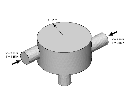
You start a new simulation in CFX-Pre and import the refined mesh. This tutorial introduces General mode (the mode used for most tutorials) in CFX-Pre. The physics for this tutorial are the same as for Simulating Flow in a Static Mixer Using CFX in Stand-alone Mode; therefore, you can import the physics settings used in that tutorial to save time.
Create a working directory.
Ansys CFX uses a working directory as the default location for loading and saving files for a particular session or project.
Download the
static_mixer_refined_mesh.zipfile here .Unzip
static_mixer_refined_mesh.zipto your working directory.Ensure that the following tutorial input files are in your working directory:
StaticMixerRefMesh.gtmStaticMixer.def(produced by following tutorial Simulating Flow in a Static Mixer Using CFX in Stand-alone Mode)StaticMixer_001.res(produced by following tutorial Simulating Flow in a Static Mixer Using CFX in Stand-alone Mode)
Set the working directory and start CFX-Pre.
For details, see Setting the Working Directory and Starting Ansys CFX in Stand-alone Mode.
The tutorial follows this general workflow for setting up the case in CFX-Pre:
In CFX-Pre, select File > New Case.
Select General in the New Case dialog box and click .
Select File > Save Case As.
Under File name, type
StaticMixerRefand click .
At least one mesh must be imported before physics are applied.
Select File > Import > Mesh.
The Import Mesh dialog box appears.
Configure the following setting(s):
Setting
Value
Files of type
CFX Mesh (*gtm *cfx)
File name
StaticMixerRefMesh.gtm [a]
Click .
The Mesh tree shows the regions in the
StaticMixerRefMesh.gtmassembly in a tree structure. The first tree branch displays the 3D regions and the level below each 3D region shows the 2D regions associated with it. The check box next to each item in theMeshtree indicates the visibility status of the object in the viewer; you can click these to toggle visibility.Note: An assembly is a group of mesh regions that are topologically connected. Each assembly can contain only one mesh, but multiple assemblies are permitted.
Right-click a blank area in the viewer and select Predefined Camera > Isometric View (Z up) from the shortcut menu.
Because the physics and region names for this simulation are
very similar to that for Tutorial 1, you can save time by importing
the settings used there. You will be importing CCL from Tutorial 1
that contains settings that reference mesh regions. For example, the
outlet boundary condition references the mesh region named out. In this tutorial, the name of the mesh regions are
the same as in Tutorial 1, so you can import the CCL without error.
Select File > Import > CCL.
The Import CCL dialog box appears.
Under Import Method, select Replace.
Replace is useful if you have defined physics and want to update or replace them with newly imported physics.
Under Files of type, select
CFX-Solver input files (*def *res).Select
StaticMixer.def.Click .
View the Outline tab.
The tree view displays a summary of the current simulation in a tree structure. Some items may be recognized from Tutorial 1; for example the boundary condition objects
in1,in2, andout.
Note:
If you import CCL that references nonexistent mesh regions, you will get errors.
A number of file types can be used as sources to import CCL, including:
Simulation files (
*.cfx)Results files (
*.res)CFX-Solver input files (
*.def)
The physics for a simulation can be saved to a CCL file at any time by selecting File > Export > CCL.
It is useful to review the options available in General mode.
Various domain settings can be set. These include:
Basic Settings
Specifies the location of the domain, coordinate frame settings and the fluids/solids that are present in the domain. You also reference pressure, buoyancy and whether the domain is stationary or rotating. Mesh motion can also be set.
Fluid Models
Sets models that apply to the fluid(s) in the domain, such as heat transfer, turbulence, combustion, and radiation models. An option absent in Tutorial 1 is Turbulent Wall Functions, which is set to Scalable. Wall functions model the flow in the near-wall region. For the k-epsilon turbulence model, you should always use scalable wall functions.
Initialization
Sets the initial conditions for the current domain only. This is generally used when multiple domains exist to enable setting different initial conditions in each domain, but can also be used to initialize single-domain simulations. Global initialization allows the specification of initial conditions for all domains that do not have domain-specific initialization.
In the Outline tree view, under
Simulation>Flow Analysis 1, double-clickDefault Domain.The domain
Default
Domain
is opened for editing.Click the Basic Settings tab and review, but do not change, the current settings.
Click Fluid Models and review, but do not change, the current settings.
Click Initialization and review, but do not change, the current settings.
Click .
For the k-epsilon turbulence model, you must specify the turbulent
nature of the flow entering through the inlet boundary. For this simulation,
the default setting of Medium (Intensity = 5%) is used. This is a sensible setting if you do not know the turbulence
properties of the incoming flow.
Under
Default Domain, double-clickin1.Click the Boundary Details tab and review the settings for Flow Regime, Mass and Momentum, Turbulence and Heat Transfer.
Click .
Solver Control parameters control aspects of the numerical-solution generation process.
In Tutorial 1 you set some solver control parameters, such as Advection Scheme and Timescale Control, while other parameters were set automatically by CFX-Pre.
In this tutorial, High Resolution is used for the advection scheme. This is more accurate than the Upwind Scheme used in Tutorial 1. You usually require a smaller time step when using this model. You can also expect the solution to take a higher number of iterations to converge when using this model.
Select Insert > Solver > Solver Control from the menu bar or click Solver Control
 .
.Configure the following setting(s):
Tab
Setting
Value
Basic Settings
Advection Scheme
> Option
High Resolution
Convergence Control
> Max. Iterations [a]
150
Convergence Control
> Fluid Timescale Control
> Timescale Control
Physical Timescale
Convergence Control
> Fluid Timescale Control
> Physical Timescale
0.5 [s]
Click .
Click the Dynamic Model Control tab.
Tip: To select Dynamic Model Control you might need to click the navigation icons next to the tabs to move ‘forward’ or ‘backward’ through the various tabs.
Ensure that Global Dynamic Model Control is selected.
Click .
Once all boundaries are created you move from CFX-Pre into CFX-Solver.
The simulation file, StaticMixerRef.cfx, contains the simulation definition in a format that can be loaded
by CFX-Pre, enabling you to complete (if applicable), restore, and
modify the simulation definition. The simulation file differs from
the CFX-Solver input file in two important ways:
The simulation file can be saved at any time while defining the simulation.
The CFX-Solver input file is an encapsulated set of meshes and CCL defining a solver run, and is a subset of the data in the simulation file.
Click Define Run
 .
.The Write Solver Input File dialog box is displayed.
If required, set the path to your working directory.
Configure the following setting(s):
Setting
Value
File name
StaticMixerRef.def
Click .
The CFX-Solver input file (
StaticMixerRef.def) is created. CFX-Solver Manager automatically starts and, on the Define Run dialog box, Solver Input File is set.If you are notified in CFX-Pre that the file already exists, click Overwrite.
Quit CFX-Pre, saving the simulation (
.cfx) file.
Two windows are displayed when CFX-Solver Manager runs. There is an adjustable split between the windows that is oriented either horizontally or vertically, depending on the aspect ratio of the entire CFX-Solver Manager window (also adjustable).
The tutorial follows this general workflow for generating the solution in CFX-Solver Manager:
In CFX-Solver Manager, the Define Run dialog box
is visible and Solver Input File has automatically
been set to the CFX-Solver input file from CFX-Pre: StaticMixerRef.def.
Configure the settings so that the results from Tutorial 1 (contained
in StaticMixer_001.res) will be used
to initialize the solution:
Under the Initial Values tab, select Initial Values Specification.
Set Initial Values Specification > Initial Values > Initial Values 1 > Initial Values 1 Settings > File Name to
StaticMixer_001.res.If you did not complete the first tutorial, you can use
StaticMixer_001.resfrom your working directory.Set Use Mesh From to
Solver Input File.Clear Initial Values Specification > Continue History From.
This will cause the CFX-Solver to use the results in the StaticMixer_001.res file as a basic initial guess for the solution, and will cause the iteration count to start from 1 instead of from the last iteration number in the initial values file.
Click Start Run.
Note: Convergence information is plotted once the second outer loop iteration is complete.
When the run is finished, specific information appears in the text window of CFX-Solver Manager.
To confirm that results interpolation was successful, look in the text window in CFX-Solver Manager. The following text appears before the convergence history begins:
+----------------------------------------------------------+
| Initial Conditions Supplied by Fields in the Input Files |
+----------------------------------------------------------+
This lists the variables that were interpolated from the results file.
After the final iteration, a message similar to the following content appears in a message window:
StaticMixerRef_001 has completed normally.
Run concluded at: Fri Nov 27 11:57:57 2009
This indicates that CFX-Solver has successfully calculated the solution for the problem to the specified accuracy or has run out of coefficient loops.
In the Solver Run Finished Normally window, ensure that the check box next to Post-Process Results is cleared to prevent CFD-Post from launching at this time.
Click .
Review the CFX-Solver Manager's Out File tab for details on the run results.
Once CFX-Solver has finished, you can use CFD-Post to review the finished results.
On the CFX-Solver Manager, select Tools > Post-Process Results or click Post-Process Results
 in the toolbar.
In the Start CFD-Post dialog box, next to Results File, ensure that
StaticMixerRef_001.resis set. If it is not, click Browse and select
 StaticMixerRef_001.res(located in the working directory).If using CFX-Solver in stand-alone mode, select Shut down CFX-Solver Manager.
This forces stand-alone CFX-Solver to close. This option is not required in Workbench.
Click .
After a short pause, CFD-Post starts.
In the following sections, you will explore the differences between the mesh and the results from this tutorial and Tutorial 1.
More information exists for use by CFD-Post in this tutorial than in Tutorial 1 because the slice plane is more detailed.
Once a new slice plane is created it can be compared with Tutorial 1. There are three noticeable differences between the two slice planes.
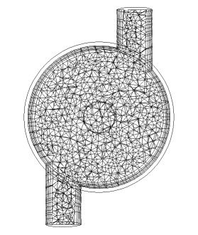
Around the edges of the mixer geometry there are several layers of narrow rectangles. This is the region where the mesh contains prismatic elements (which are created as inflation layers). The bulk of the geometry contains tetrahedral elements.
There are more lines on the plane than there were in Tutorial 1. This is because the slice plane intersects with more mesh elements.
The curves of the mixer are smoother than in Tutorial 1 because the finer mesh better represents the true geometry.
Right-click a blank area in the viewer and select Predefined Camera > Isometric View (Z up).
From the menu bar, select Insert > Location > Plane or under Location, click Plane.
In the Insert Plane dialog box, type
Sliceand click .The Geometry, Color, Render and View tabs enable you to switch between settings.
Configure the following setting(s):
Tab
Setting
Value
Geometry Domains
Default
Domain
Definition
> Method
XY Plane
Definition
> Z
1 [m]
Plane Type
Slice
Render
Show Faces
(Cleared)
Show Mesh Lines
(Selected)
Click .
Right-click a blank area in the viewer and select Predefined Camera > View From +Z.
If necessary, click Zoom Box
 and zoom in on the geometry to view it in greater detail.
Compare the on-screen image with the equivalent picture from Simulating Flow in a Static Mixer Using CFX in Stand-alone Mode (in the section Rendering Slice Planes).
Here, you will color the plane by temperature.
Configure the following setting(s):
Tab
Setting
Value
Color
Mode [a]
Variable
Variable
Temperature
Range
Global
Render
Show Faces
(Selected)
Show Mesh Lines
(Cleared)
Click .
In CFD-Post, you may load multiple results files into the same instance for comparison.
To load the results file from Tutorial 1, select File > Load Results or click Load Results
 .
.(Do not click until instructed to do so.) In the Load Results File dialog box, select
StaticMixer_001.resfrom your working directory.On the right side of the dialog box, there are three frames:
Case options
Additional actions
CFX run history and multi-configuration options.
Under Case options, select Keep current cases loaded and ensure that Open in new view is selected.
Under Additional actions, ensure that the Clear user state before loading check box is cleared.
Under CFX run history and multi-configuration options, ensure that Load only the last results is selected.
Click to load the results.
In the tree view, there is now a second group of domains, meshes and boundary conditions with the heading
StaticMixer_001.In the 3D Viewer, there are two viewports named View 1 and View 2; the former shows StaticMixer_001 and the latter shows StaticMixerRef_001.
Double-click the
Wireframeobject underUser Locations and Plots.In the Definition tab, set Edge Angle to
5 [degree].Click .
Click Synchronize camera in displayed views
 so that all viewports maintain the same camera
position.
so that all viewports maintain the same camera
position.Right-click a blank area in the viewer and select Predefined Camera > Isometric View (Z up).
Both meshes are now displayed in a line along the Y axis. Notice that one mesh is of a higher resolution than the other.
Set Edge Angle to
30 [degree].Click .
The visibility status of each object is maintained separately
for each viewport. This allows some planes to be shown while others
are hidden. However, you can also use the Synchronize visibility
in displayed views  to synchronize the visibility of objects that
you add.
to synchronize the visibility of objects that
you add.
Under User Locations and Plots, select the check box beside
Slice.Right-click in the viewer and select Predefined Camera > View From -Z.
Note the difference in temperature distribution.
In the viewer toolbar, click Synchronize visibility in displayed views
to deselect the option.Click in View 1 in the 3D Viewer, then clear the visibility check box for
Slicein the Outline tree view.Click in View 2. Note that the visibility check box for
Slicehas been re-selected as it describes the state of the plane for View 2. Clear the visibility check box forSlicein this view.To return to a single viewport, select the option with a single rectangle.
Ensure that the visibility check box for
Sliceis cleared.Right-click
StaticMixer_001in the tree view and select Unload.
In this part of the tutorial, you will view the mesh on the outlet. You will see five layers of inflated elements against the wall. You will also see the triangular faces of the tetrahedral elements closer to the center of the outlet.
Right-click a blank area in the viewer and select Predefined Camera > Isometric View (Z up).
In the tree view, ensure that the visibility check box for
StaticMixerRef_001>Default Domain>outis selected, then double-clickoutto open it for editing.Because the boundary location geometry was defined in CFX-Pre, the details view does not display a Geometry tab as it did for the planes.
Configure the following setting(s):
Tab
Setting
Value
Render
Show Faces
(Cleared)
Show Mesh Lines
(Selected)
Color Mode
User Specified
Line Color
(Select any light color)
Click .
Click Zoom Box
.Zoom in on the geometry to view
outin greater detail.Click Rotate
 on
the Viewing Tools toolbar.
on
the Viewing Tools toolbar.Rotate the image as required to clearly see the mesh.
To show more clearly what effect inflation has on the shape of the elements, you will use volume objects to show two individual elements. The first element that will be shown is a normal tetrahedral element; the second is a prismatic element from an inflation layer of the mesh.
Leave the surface mesh on the outlet visible to help see how surface and volume meshes are related.
From the menu bar, select Insert > Location > Volume or, under Location click Volume.
In the Insert Volume dialog box, type
Tet Volumeand click .Configure the following setting(s):
Tab
Setting
Value
Geometry
Definition
> Method
Sphere
Definition
> Point [a]
0.08, 0, -2
Definition
> Radius
0.14 [m]
Definition
> Mode
Below Intersection
Inclusive [b]
(Cleared)
Color
Color
Red
Render
Show Faces
> Transparency
0.3
Show Mesh Lines
(Selected)
Show Mesh Lines
> Line Width
1
Show Mesh Lines
> Color Mode
User Specified
Show Mesh Lines
> Line Color
Grey
Click to create the volume object.
Right-click
Tet Volumeand choose Duplicate.In the Duplicate Tet Volume dialog box, type
Prism Volumeand click .Double-click
Prism Volume.Configure the following setting(s):
Tab
Setting
Value
Geometry
Definition
> Point
-0.22, 0.4, -1.85
Definition
> Radius
0.206 [m]
Color
Color
Orange
Click .
Double-click the
Default Domain Defaultobject.Configure the following setting(s):
Tab
Setting
Value
Render
Show Faces
(Selected)
Show Mesh Lines
(Selected)
Line Width
2
Click .
You will see the layers of inflated elements on the wall of the main body of the mixer. Within the body of the mixer, there will be many lines that are drawn wherever the face of a mesh element intersects the slice plane.
From the menu bar, select Insert > Location > Plane or under Location, click Plane.
In the Insert Plane dialog box, type
Slice 2and click .Configure the following setting(s):
Tab
Setting
Value
Geometry
Definition
> Method
YZ Plane
Definition
> X
0 [m]
Render
Show Faces
(Cleared)
Show Mesh Lines
(Selected)
Click .
Turn off the visibility of all objects except
Slice 2.To see the plane clearly, right-click in the viewer and select Predefined Camera > View From -X.
You can use the Report Viewer to check the quality of your mesh.
For example, you can load a .def file into CFD-Post and
check the mesh quality before running the .def file in the solver.
Click the Report Viewer tab (located below the viewer window).
A report appears. Look at the table shown in the "Mesh Report" section.
Double-click
Report>Mesh Reportin the Outline tree view.In the Mesh Report details view, select Statistics > Maximum Face Angle.
Click Refresh Preview.
Note that a new table, showing the maximum face angle for all elements in the mesh, has been added to the "Mesh Report" section of the report. The maximum face angle is reported as 148.95°.
As a result of generating this mesh statistic for the report,
a new variable, Maximum Face Angle, has been
created and stored at every node. This variable will be used in the
next section.
In this section, you will visualize the mesh elements that have
a Maximum Face Angle value greater than 140°.
Click the 3D Viewer tab (located below the viewer window).
Right-click a blank area in the viewer and select Predefined Camera > Isometric View (Z up).
In the Outline tree view, select the visibility check box of
Wireframe.From the menu bar, select Insert > Location > Volume or under Location, click Volume.
In the Insert Volume dialog box, type
Max Face Angle Volumeand click .Configure the following setting(s):
Click .
The volume object appears in the viewer.

Next, you will create a point object to show a node that has
the maximum value of Maximum Face Angle. The
point object will be represented by a 3D yellow crosshair symbol.
In order to avoid obscuring the point object with the volume object,
you may want to turn off the visibility of the latter.
From the menu bar, select Insert > Location > Point or under Location, click Point.
Click to use the default name.
Configure the following setting(s):
Tab
Setting
Value
Geometry
Definition
> Method
Variable Maximum
Definition
> Location
Default Domain
Definition
> Variable
Maximum Face Angle
Symbol
Symbol Size
2
Click .