


This tutorial includes:
Important: This tutorial requires file TimeBladeRowIni_001.res, which is produced by following tutorial Time Transformation Method for a Transient Rotor-stator Case.
In this tutorial you will learn about:
Initializing profile data.
Expanding profile data.
Defining injection regions.
Monitoring expressions during a solver run.
Using streamlines in CFD-Post to trace the flow field starting from injection regions.
Component | Feature | Details |
|---|---|---|
CFX-Pre | Injection Regions | Circular Hole |
Cylindrical Slot | ||
Profile Data | Initialization | |
Editing | ||
Analysis Type | Transient Blade Row | |
Fluid Type | Air Ideal Gas | |
Domain Type | Multiple Domains | |
Rotating Frame of Reference | ||
Turbulence Model | Shear Stress Transport | |
Heat Transfer | Total Energy | |
Boundary Conditions | Inlet (Subsonic) | |
Outlet (Subsonic) | ||
Wall (Counter Rotating) | ||
CFD-Post | Plots | Contour |
Point Cloud | ||
Injection Region | ||
Streamline |
This tutorial models film cooling in a turbine using the Injection Regions feature of CFX.
You will build upon the geometry and setup of tutorial Time Transformation Method for a Transient Rotor-stator Case, adjusting the inlet temperature and adding injection regions to the rotor and hub. Near the end of this tutorial, you will produce a contour plot and streamlines to show the effect of injecting relatively cool air through the injection regions.
If this is the first tutorial you are working with, it is important to review the following topics before beginning:
Create a working directory.
Ansys CFX uses a working directory as the default location for loading and saving files for a particular session or project.
Download the
film_cooling.zipfile here .Unzip
film_cooling.zipto your working directory.Ensure that the following tutorial input files are in your working directory:
FCInjectionPositions.csvTBRInletProfile.csvTBROutletProfile.csvTBRTurbineRotor.gtmTBRTurbineStator.gtmTimeBladeRowIni_001.res(produced by following tutorial Time Transformation Method for a Transient Rotor-stator Case)
Set the working directory and start CFX-Pre.
For details, see Setting the Working Directory and Starting Ansys CFX in Stand-alone Mode.
Open the results file named
TimeBladeRowIni_001.res.Save the case as
FilmCooling.cfxin your working directory.
Adjust the inlet temperature as follows:
Edit
S1 Inlet.On the Boundary Details tab, set Heat Transfer > Total Temperature to
1000 [K].Click OK.
File FCInjectionPositions.csv is a profile data file that contains information about specific injection positions. You can optionally view this file’s contents using a text editor. The file contains 3 function definitions, each consisting of a name, optional parameter data, a declaration of the spatial field variables, and table data. Note that the function names, parameter names, and table column labels must be CEL-compatible; these names may contain spaces but must not contain the underscore character or any symbols.
Load FCInjectionPositions.csv:
Select Tools > Initialize Profile Data.
The Initialize Profile Data dialog box appears.
Beside Profile Data File, click Browse
 .
.The Select Profile Data File dialog box appears.
Select FCInjectionPositions.csv and click Open.
In the Initialize Profile Data dialog box, select all three Visibility check boxes so that, in the viewer, symbols will appear at the (planned) injection positions.
Note that the symbol visibility can also be controlled in the Outline tree view by selecting or clearing the check boxes under
Simulation>Expressions, Functions and Variables>User Functions.Click OK.
The profile data is loaded and initialized. Note that an additional three profile functions appear in the Outline tree view, under
Simulation>Expressions, Functions and Variables>User Functions:Hub CoolingRotor Pressure Surface CoolingRotor Suction Surface Cooling
As an exercise, change the appearance of the user function symbols:
In the Outline tree view, right-click
Simulation>Expressions, Functions and Variables>User Functions>Hub Coolingand select Render > Properties.The Render Options - User Function Hub Cooling dialog box appears.
Set Symbol to
Ball.Set Symbol Size to
0.5.Click OK.
In the viewer, the symbols that mark the injection positions (cooling hole locations) on the hub are now shown as balls.
Using the same procedure, change the shape and size of the user function symbols that show the injection positions on the rotor pressure and suction surfaces.
If the curled-arrow symbols that mark interfaces are shown in the viewer, hide them by right-clicking the viewer background and deselecting Markers > Interface.
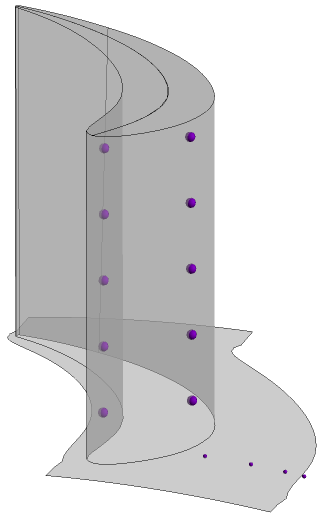
Note that, as shown in Figure 38.1: Injection Positions, one of the injection positions on the hub is slightly outside the modeled passage; any such injection position is effectively relocated (by the CFX-Solver) to a corresponding position between the periodic interfaces. You can therefore create injection positions without having to know the exact locations of the periodic interfaces.
Note:
If the injection positions (cooling hole locations) require rotation, added instances, or other transformations, you can use the Edit Profile Data dialog box to edit the profile data file. For details, see Edit Profile Data in the CFX-Pre User's Guide.
If you are editing the profile data with an application other than CFX-Pre or a plain text editor, ensure that you preserve a reasonable number of significant digits in the data.
In the previous section, you noted that one of the injection positions is slightly outside the modeled passage.
Later in this tutorial, there is a postprocessing demonstration that requires a modified copy of the profile that, within the modeled passage in particular, has all of the modeled injection positions. Such a profile can be made by expanding the original profile to cover two passages.
Create an expanded version of the profile as follows:
Select Tools > Edit Profile Data.
The Edit Profile Data dialog box appears.
Under Source Profile, click Browse
.The Select Profile Data File dialog box appears.
From your working directory, select FCInjectionPositions.csv and click Open.
In the Edit Profile Data dialog box, set Write to Profile to FCInjectionPositions_2p.csv.
IMPORTANT: Ensure that Initialize New Profile After Writing is cleared in order to prevent the profile data from being initialized with the expanded profile.
In the Transformations frame, click Add new item
 , set Name to
 Transformation 1, and click OK.Configure the following setting(s):
Setting
Value
Transformation 1
> Option
Expansion
Transformation 1
> Expansion Definition
> Rotation Option
Principal Axis
Transformation 1
> Expansion Definition
> Axis
Z
Transformation 1
> Expansion Definition
> Passages in Profile
1
Transformation 1
> Expansion Definition
> Passages in 360
42
Transformation 1
> Expansion Definition
> Expansion Option
Spec. Number of Passages
Transformation 1
> Expansion Definition
> Pass. in Expansion
2
Transformation 1
> Expansion Definition
> Theta Offset
-8.57143 [degree]
Click .
The new profile (which is not applied to the simulation, but which is available as file FCInjectionPositions_2p.csv) covers two passages, and will be used in the postprocessing section of this tutorial. Although the expanded profile contains many unneeded points outside the modeled passage, it (importantly) contains all of the injection positions within the modeled passage.
As a best practice, you will create associations between the user function data and injection region settings. This will prepare CFX-Pre to automatically configure many of the injection region settings later in this tutorial. Note that these associations are not required; you can always choose to specify any or all of the injection region settings manually.
Edit the three relevant user functions as follows:
In the Outline tree view, right-click
Simulation>Expressions, Functions and Variables>User Functions>Hub Coolingand select Edit.Under Parameters, select MassFlow (in the list).
Select MassFlow > Parameter List.
Set Parameter List to
Injection Mass Flow Rate.Also make the following associations for user function
Hub Cooling:With Value Fields set to
Cooling Temperature, select Cooling Temperature > Parameter List, then set Parameter List toStationary Frame Total Temperature.With Value Fields set to
Hole Diameter, select Hole Diameter > Parameter List, then set Parameter List toDiameter.
Click OK.
Make the following associations for user function
Rotor Pressure Surface Cooling(clicking OK when done):With Parameters set to
Diameter, ensure that Parameter List is set toDiameter.With Parameters set to
InjectionTemperature, set Parameter List toStationary Frame Total Temperature.With Value Fields set to
Mass Flow, set Parameter List toInjection Mass Flow Rate.
Make the same associations for user function
Rotor Suction Surface Coolingas for user functionRotor Pressure Surface Cooling(clicking OK when done).
Now that you have initialized the profile data and have created associations between the profile data and injection region settings, you are ready to use the profile data to create cooling holes.
Add cooling holes to the rotor as follows:
Select Insert > Injection Region > in R1.
The Insert Injection Region dialog box appears.
Set Name to
Rotor Pressure Surface Cooling Holesand click OK.Configure the following setting(s):
Tab
Setting
Value
Basic Settings Region Type
Inlet
Injection Location Type
> Option
Selected 2D Regions
Injection Location Type
> Location
BLADE 2
Injection Positions
> Option
From Profile
Injection Positions
> Profile Name
Rotor Pressure Surface Cooling
Injection Positions
> Generate Values
(Click)
This fills in settings on the Injection Details tab using the associations that you defined earlier in the
Rotor Pressure Surface Coolinguser function.Coordinate Frame
Coord 0
Frame Type
Rotating
Injection Details
Injection Model
> Option
Circular Hole
Injection Model
> Diameter
Rotor Pressure Surface Cooling.Diameter()
Mass And Momentum
> Option
Injection Mass Flow Rate
Mass and Momentum
> Mass Flow Rate
Rotor Pressure Surface Cooling.Mass Flow(x,y,z)
Mass and Momentum
> Mass Flow Rate Area
Per Injection Position
Flow Direction
> Option
Normal to Boundary Condition
Heat Transfer
> Option
Stationary Frame Total Temperature
Heat Transfer
> Stat. Frame Tot. Temp
Rotor Pressure Surface Cooling.InjectionTemperature()
Click OK.
The injection region is listed in the Outline tree view, under the applicable domain.
In the viewer, symbols representing the cooling holes
appear on the rotor pressure surface. You can optionally adjust
the rendering properties of injection region
Rotor Pressure Surface Cooling Holes
by right-clicking it in the Outline tree view and
selecting Render > Properties.
Note that the Symbol option Injection Shape is particularly recommended because
the resulting symbols (wherever possible) show not only the position, but also the orientation, shape, and size, of each cooling hole.
Additional settings for visualizing an injection region are available in
the details view, on the Plot Options tab.
You can optionally turn off the visibility of user function
Rotor Pressure Surface Cooling.
Using the same procedure, add an injection region, Rotor Suction Surface Cooling Holes, for the
cooling holes on the rotor suction surface, using the Rotor Suction Surface Cooling
profile data for the injection positions, diameter, mass flow, and temperature.
You can optionally turn off the visibility of user function
Rotor Suction Surface Cooling.
Add cooling holes to the hub as follows:
Select Insert > Injection Region > in R1.
The Insert Injection Region dialog box appears.
Set Name to
Hub Cooling Holesand click OK.Configure the following setting(s):
Tab
Setting
Value
Basic Settings Region Type
Inlet
Injection Location Type
> Option
Selected 2D Regions
Injection Location Type
> Location
Entire HUB 2
Injection Positions
> Option
From Profile
Injection Positions
> Profile Name
Hub Cooling
Injection Positions
> Generate Values
(Click)
This fills in settings on the Injection Details tab using the associations that you defined earlier in the
Hub Coolinguser function.Coordinate Frame
Coord 0
Frame Type
Rotating
Injection Details
Injection Model
> Option
Circular Hole
Injection Model
> Diameter
Hub Cooling.Hole Diameter(x,y,z)
Mass And Momentum
> Option
Injection Mass Flow Rate
Mass and Momentum
> Mass Flow Rate
Hub Cooling.MassFlow()
Mass and Momentum
> Mass Flow Rate Area
As Specified
(This indicates that the specified mass flow rate is the total over all 4 modeled holes on the hub.)
Flow Direction
> Option
Normal to Boundary Condition
Heat Transfer
> Option
Stationary Frame Total Temperature
Heat Transfer
> Stat. Frame Tot. Temp
Hub Cooling.Cooling Temperature(x,y,z)
Click OK.
You can optionally turn off the visibility of user function
Hub Cooling.
Add a cylindrical slot to the hub as follows:
Create a user line (Insert > User Locations > User Line) named
User Line 1, with Option set toTwo Points, Number of Points set to 2, Point 1 set to (-0.245, 0.001, 0.21), and Point 2 set to (-0.243, -0.026, 0.21).This user line marks the position and orientation of the slot.
Note that the user line visibility can be controlled in the Outline tree view by selecting or clearing the check box for
Simulation>User Locations>User Line 1.Select Insert > Injection Region > in R1.
The Insert Injection Region dialog box appears.
Set Name to
Platform Cooling Slotand click OK.Configure the following setting(s):
Tab
Setting
Value
Basic Settings Region Type
Inlet
Injection Location Type
> Option
Selected 2D Regions
Injection Location Type
> Location
Entire HUB 2
Injection Positions
> Option
User Location
Injection Positions
> User Location List
User Line 1
Coordinate Frame
Coord 0
Frame Type
Rotating
Injection Details
Injection Model
> Option
Cylindrical Slot
Injection Model
> Slot Width
1 [mm]
Injection Model
> Axis Definition
> Option
From Domain
Mass And Momentum
> Option
Injection Mass Flow Rate
Mass and Momentum
> Mass Flow Rate
1.5e-3 [kg s^-1]
Mass and Momentum
> Mass Flow Rate Area
As Specified
(This indicates that the specified mass flow rate applies over the slot as specified for the modeled sector of the wheel.)
Flow Direction
> Option
Normal to Boundary Condition
Heat Transfer
> Option
Stationary Frame Total Temperature
Heat Transfer
> Stat. Frame Tot. Temp
420 [K]
Click OK.
In the viewer, a line drawing representing the cylindrical slot
appears on the hub. You can optionally adjust
the rendering properties of injection region
Platform Cooling Slot
by right-clicking it in the Outline tree view and
selecting Render > Properties.
Additional settings for visualizing an injection region are available in
the details view, on the Plot Options tab.
An injection region can serve as a locator in a CEL expression in CFX-Pre and in CFX-Solver. Such an expression could be used, for example, to create a solver monitor.
As an exercise, create a solver monitor that monitors an expression for the area average of pressure on the hub cooling holes.
Select Insert > Solver > Output Control.
The Output Control details view appears.
On the Monitor tab, under Monitor Points and Expressions, click Add new item
.The Insert Monitor Point dialog box appears.
Set Name to
Average Pressure on Hub Cooling Holesand click OK.Under Monitor Points and Expressions > Average Pressure on Hub Cooling Holes:
Set Option to
Expression.Set Expression Value to
areaAve(Pressure)@Hub Cooling Holes.
Click Apply.
As an exercise, create the following monitors that will be used later in this tutorial to confirm that there is conservation of mass in the rotor passage:
Monitor Name | Expression Value |
|---|---|
Rotor Pressure Surface Cooling Hole Mass Flow | massFlow()@Rotor Pressure Surface Cooling Holes |
Rotor Suction Surface Cooling Hole Mass Flow | massFlow()@Rotor Suction Surface Cooling Holes |
Hub Cooling Hole Mass Flow | massFlow()@Hub Cooling Holes |
Platform Cooling Slot Mass Flow | massFlow()@Platform Cooling Slot |
Rotor Passage Inlet Mass Flow | massFlow()@REGION:Entire INFLOW 2 |
Rotor Passage Outlet Mass Flow | massFlow()@REGION:Entire OUTFLOW 2 |
Net Flow into Rotor Passage | massFlow()@Rotor Pressure Surface Cooling Holes + massFlow()@Rotor Suction Surface Cooling Holes + massFlow()@Hub Cooling Holes + massFlow()@Platform Cooling Slot + massFlow()@REGION:Entire INFLOW 2 + massFlow()@REGION:Entire OUTFLOW 2 |
Because the current case was built upon the results of another case, a definition file (*.def) name is stored in the Execution Control settings. Update that name to reflect the current case as follows:
Click Execution Control
 .
.Configure the following setting(s):
Tab
Setting
Value
Run Definition
Input File Settings
> Solver Input File
FilmCooling.def [a]
Confirm that the rest of the execution control settings are set appropriately.
Click .

In CFX-Solver Manager, ensure that the Define Run dialog box is displayed.
Under the Initial Values tab, select Initial Values Specification.
Under Initial Values Specification > Initial Values, select
Initial Values 1.Under Initial Values Specification > Initial Values > Initial Values 1 Settings > File Name, click Browse
.Select
TimeBladeRowIni_001.resfrom your working directory.Click Open.
Click Start Run.
CFX-Solver runs and attempts to obtain a solution.
As an exercise, show each injection region's mass flow in a new monitor plot:
In the CFX-Solver Manager, select Workspace > New Monitor.
The New Monitor dialog box appears.
Set Name to
Injection Regions.Set Type to
Plot Monitor.Click OK.
The Monitor Properties: Injection Regions dialog box appears.
In the dialog box, on the Plot Lines tab, in the tree starting with
Plot Line Variable, expand FLOW >INJECTION REGION, then select the following:Hub Cooling Holes>P-Mass Injection Region Flow on Hub Cooling Holes (R1)Platform Cooling Slot>P-Mass Injection Region Flow on Platform Cooling Slot (R1)Rotor Pressure Surface Cooling Holes>P-Mass Injection Region Flow on Rotor Pressure Surface Cooling Holes (R1)Rotor Suction Surface Cooling Holes>P-Mass Injection Region Flow on Rotor Suction Surface Cooling Holes (R1)
Click OK.
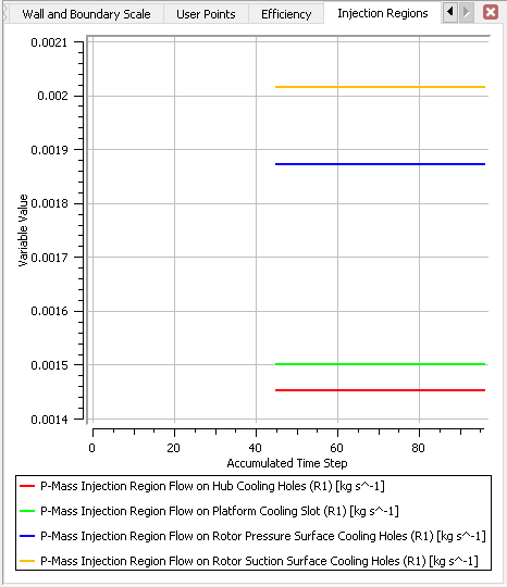
As shown in Figure 38.2: Mass Flows through Injection Regions, a new monitor plot appears in the CFX-Solver Manager showing four horizontal lines; these lines correspond to the total mass flows through:
The 4 hub cooling holes
The hub cooling slot
The 5 rotor pressure surface cooling holes
The 5 rotor suction surface cooling holes.
Show the monitors that you created earlier, in CFX-Pre:
Click the User Points tab.
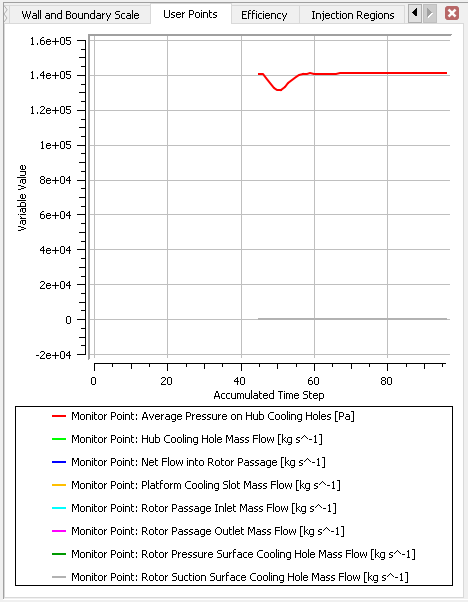
Observe that the monitor Average Pressure on Hub Cooling Holes is plotted against
Accumulated Time Step, as shown by the topmost plot line in Figure 38.3: User Points versus Accumulated Time Step.The other monitors that you defined are also shown, but not currently at an appropriate scale for viewing.
Right-click inside the User Points tab and select Monitor Properties.
The Monitor Properties: User Points dialog box appears.
In the dialog box, on the Plot Lines tab, clear
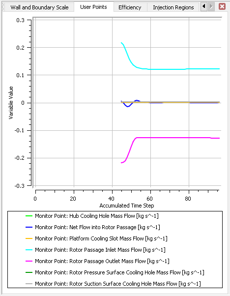
USER POINT>Average Pressure on Hub Cooling Holes, then click OK.With the plot line Average Pressure on Hub Cooling Holes omitted, the chart is now re-scaled so that the remaining plot lines are easier to see, as shown in Figure 38.4: Conservation-related User Points versus Accumulated Time Step. The plot line
Net Flow into Rotor Passageapproaches zero, indicating that mass flow is conserved in the rotor passage, as expected.
At the end of the run, a dialog box is displayed stating that the simulation has ended.
When CFX-Solver is finished, select the check box next to Post-Process Results.
If using stand-alone mode, select the check box next to Shut down CFX-Solver Manager.
Click .
In the following sections, you will:
Show the mesh lines in the rotor domain.
Create a contour plot that shows the temperature on the rotor and hub.
Use the expanded profile data that you prepared earlier (FCInjectionPositions_2p.csv) to create point clouds that represent injection positions, specifically the cooling hole centers.
Adjust coloring and rendering options for injection regions.
Plot streamlines that originate from injection regions.
Perform quantitative calculations on an injection region.
In the Outline tree view, select the check boxes for
R1 BladeandR1 Hub.Edit
R1 Blade.In the details view, on the Render tab, clear Show Faces, select Show Mesh Lines, and click Apply.
Edit
R1 Hubsimilarly.Turn off the visibility of
User Locations and Plots>Wireframe.
Click Insert > Contour and accept the default name.
Configure the following setting(s):
Tab
Setting
Value
Geometry
Locations
R1 Blade,R1 Hub
Variable
Temperature
Range
Global
# of Contours
21
Render
Show Contour Bands
> Lighting
(Cleared)
Click .
The contour plot shows Temperature values
on the rotor and hub. As shown in Figure 38.5: Temperature on Blade and Hub, the
effect of film cooling is apparent.
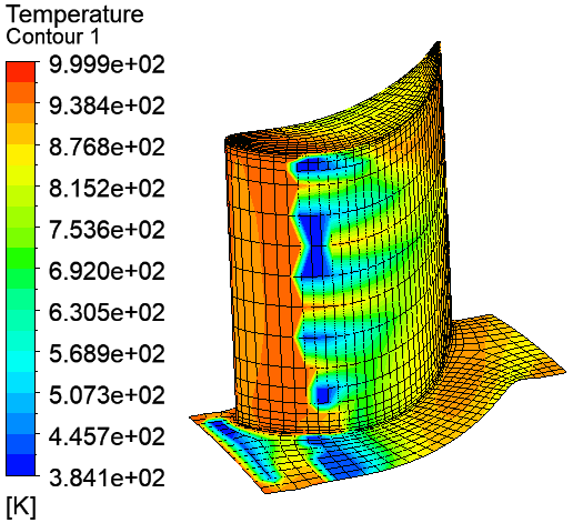
Increasing the mesh resolution would better resolve the circular shape of the cooling holes. A case with film cooling is typically simulated using a finer mesh than used here. As a best practice, there should be 3 to 5 elements across the hole diameter for any given cooling hole. As expected, flow quantities are conserved, regardless of the mesh resolution.
Note: For a coarse mesh in which the mesh faces at an injection position are larger than the hole size,
you must set, in the Solver Control details view, on the Advanced
Options tab, Injection Control > Surface Injection
Control > Surface Overlap Type to Nearest Face.
Note that, as a side effect of using this option, each cooling hole is resolved by only one
mesh face. Also note that, under this option, any given mesh face is permitted to resolve multiple
cooling holes.
In this section, you will begin by creating point clouds that show the cooling hole centers. To ensure that every cooling hole center on the hub is represented, including the one (as mentioned earlier) specified by a position outside the mesh (the corresponding position in an adjacent flow passage), you will use the expanded profile (created earlier) to create the point clouds.
You will then use injection region object Rotor Suction Surface Cooling Holes
to visualize the approximate shape of the cooling holes on the rotor suction surface.
Create the point clouds using the expanded profile that you prepared earlier:
Select File > Import > Import Surface, Line or Point Data.
The Import Surface, Line or Point Data dialog box appears.
Set File to FCInjectionPositions_2p.csv.
Set Import As to
Point Cloud.Click OK.
In the Outline tree view, under
User Locations and Plots, three point cloud objects appear. These objects correspond to the three profile data sets inFCInjectionPositions_2p.csv, which represent all cooling hole locations (in two passages) for the hub, rotor pressure surface, and rotor suction surface.Edit
User Locations and Plots>Imported Hub Cooling.In the details view, on the Symbol tab, set Symbol to
Balland Symbol Size to0.25.Click Apply.
The viewer shows ball symbols at the cooling hole locations on the hub.
Change the symbols similarly for the other two point cloud objects.
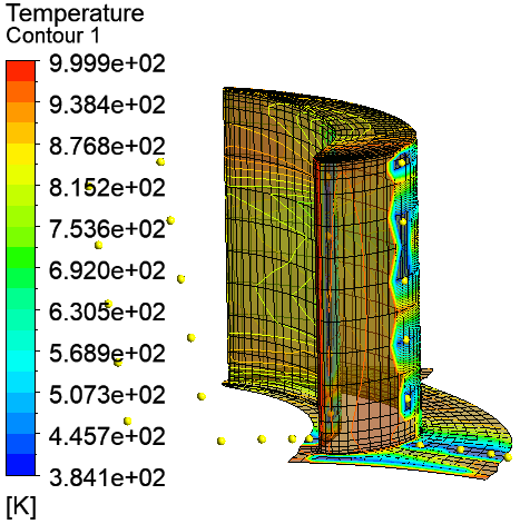
You should see all cooling hole locations inside the modeled passage (as well as many outside the passage), as shown in Figure 38.6: Hole Locations shown using Point Cloud (which has transparency applied to the contour plot to help show the symbols).
Color injection region Rotor Suction Surface Cooling Holes
using variable Rotor Suction Surface Cooling Holes Area Fraction
to help resolve the shapes of the cooling holes on the rotor suction surface, as follows:
Turn off the visibility of contour plot
Contour 1.Turn on the visibility of injection region
Rotor Suction Surface Cooling Holes.Edit injection region
Rotor Suction Surface Cooling Holes.In the details view, on the Color tab, change Mode to
Variableand, using the Ellipsis icon, change
Variable to
icon, change
Variable to Rotor Suction Surface Cooling Holes Area Fraction.Click Apply.
The approximate shapes of the cooling holes, as shown by
injection region Rotor Suction Surface Cooling Holes,
are in agreement with the hole center positions, as
marked by the corresponding point cloud.
Injection region Rotor Suction Surface Cooling Holes includes all
of the mesh faces that meet or overlap the injection holes in the injection region.
By default, the rendering is trimmed at a certain value of the injection region's area fraction variable.
As an exercise, adjust the rendering to be trimmed at an area fraction of 0.25:
Edit injection region
Rotor Suction Surface Cooling Holes.In the details view, on the Render tab, ensure that Use Post Region Rendering is selected and set Area Fraction to
0.25.Click Apply.
The injection region is now clipped at an Area Fraction value of 0.25;
the portion of the injection region that remains visible is the portion that has area fraction variable
Rotor Suction Surface Cooling Holes Area Fraction greater than the specified
value of 0.25.
Note: The Use Post Region Rendering setting works independently of the coloring settings. In this tutorial, coloring the injection region by its area fraction variable happened to help illustrate that clipping occurs at the specified value of Area Fraction.
In this section, you will produce streamlines that start from the injection regions, specifically the vertices of the mesh faces that resolve the cooling holes and slot.
From the main menu, select Insert > Streamline.
The Insert Streamline dialog box appears.
Accept the default name and click .
Set Definition > Start From to a selection of all four injection regions:
Hub Cooling HolesPlatform Cooling SlotRotor Pressure Surface Cooling HolesRotor Suction Surface Cooling Holes
Set Definition > Sampling to
Vertex.To help ensure that every injection position in the passage has associated streamlines, set Definition > Reduction to
Reduction Factorand Definition > Factor to1.0.Set Definition > Boundary Data to Hybrid.
Ensure that Cross Periodics is selected.
This setting enables the streamlines to cross periodic boundaries.
Click the Color tab.
Set Mode to
Variable.Set Variable to
Temperature.Set Range to
Global.Click the Symbol tab.
Ensure that Show Streams is selected.
Set Show Streams > Stream Type to
Tube.Set Show Streams > Tube Width to
1.0.Click Apply.
Streamlines start from each injection region in the passage, as shown in Figure 38.7: Streamlines starting from Injection Regions.
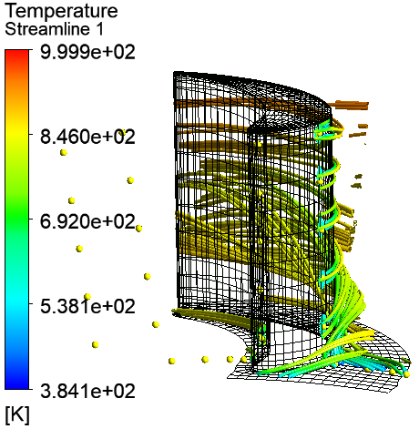
Note that, when using a coarse mesh (as in this tutorial), and depending on the size and distribution of the injection holes/slots, some injection positions might not have adequate graphical representation; without adequate graphical representation, there could be fewer/no streamlines originating from an injection position (when plotting streamlines from the injection region).
For the current case, to improve rendering of the injection holes/slot
(thereby increasing the number of streamlines plotted) you can try adjusting
the area fractions used to clip the rendered injection regions. In
Showing the Cooling Hole Locations, you have already adjusted the area fraction
used to clip injection region Rotor Suction Surface Cooling Holes.
Using the same technique, adjust the area fraction used to clip the following two
other injection regions, using the indicated Area Fraction values:
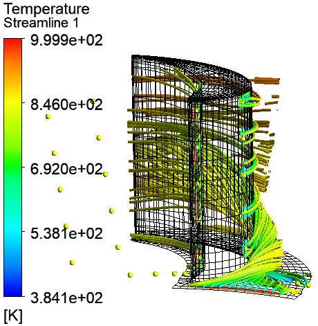
Rotor Pressure Surface Cooling Holes: Area Fraction = 0.16Platform Cooling Slot: Area Fraction = 0.1
Note: Due to a Bug that affects the rendering of injection regions in Release 2024 R2 of CFD-Post, you might need to turn off (being sure to click Apply) the Use Post Region Rendering option (in the details view, on the Render tab) for the applicable injection region(s), then turn on (being sure to click Apply) the Use Post Region Rendering option for the same injection region(s).
The holes and slot are now better resolved for these two injection regions, as shown in Figure 38.8: Injection Regions Clipped at Lower Area Fractions. Note the appearance of additional streamlines on these regions.
You can calculate quantities on an injection region, either via CCL or via the function calculator. When using an injection region in a calculation in CFD-Post, the injection region effectively consists of only the holes/slots; the remainder of the 2D region used to define the injection region is excluded.
Important: A Bug that affects Release 2024 R2 of CFD-Post causes inaccurate calculations on injection regions in multidomain cases. The suggested workaround is to turn on (being sure to click Apply) the Use Post Region Rendering option (in the details view, on the Render tab) for the applicable injection region(s), then turn off (being sure to click Apply) the Use Post Region Rendering option for the same injection region(s), then recalculate any previously computed results.
As an exercise, use the Function Calculator to calculate quantities
that apply to all holes, taken collectively, of injection region Hub Cooling Holes:
Apply the Bug workaround just mentioned for injection region
Hub Cooling Holesby turning on, then off, its Use Post Region Rendering option:Edit injection region
Hub Cooling Holes.In the details view, on the Render tab, ensure that Use Post Region Rendering is turned on.
Click Apply.
In the details view, on the Render tab, turn off Use Post Region Rendering.
Click Apply.
You are now ready to calculate quantities on injection region
Hub Cooling Holes.
Calculate the mass flow that passes through all holes, taken collectively, of injection region
Hub Cooling Holesas follows:Select Tools > Function Calculator.
In the Function Calculator, set Function to
massFlowand Location toHub Cooling Holes.Click Calculate.
The computed mass flow appears under Results.
Calculate the mass flow integral of static enthalpy over all holes, taken collectively, of injection region
Hub Cooling Holesas follows:In the Function Calculator, set Function to
massFlowInt, Location toHub Cooling Holes, and Variable toStatic Enthalpy.Click Calculate.
The computed integral appears under Results.
Calculate the area of all holes, taken collectively, of injection region
Hub Cooling Holesas follows:In the Function Calculator, set Function to
areaand Location toHub Cooling Holes.Click Calculate.
The computed area appears under Results.
Note that area-dependent results are approximate, being affected by mesh coarseness as well as the geometric fidelity of the approximate (polygonal) geometry used internally to represent the cooling holes.