


This tutorial includes:
In this tutorial you will learn about:
Controlling a simulation with operating points.
Working with operating map charts in CFD-Post.
Component | Feature | Details |
|---|---|---|
CFX-Pre | User Mode | General mode |
Analysis Type | Steady State | |
Fluid Type | Air Ideal Gas | |
Domain Type | Single Domain | |
Turbulence Model | Shear Stress Transport | |
Heat Transfer | Total Energy | |
Boundary Conditions | Inlet (Subsonic) | |
Outlet (Subsonic) | ||
Wall: No-Slip | ||
Wall: Adiabatic | ||
Timescale | Physical Timescale | |
CFX-Solver Manager | Define Run Dialog Box | Operating Points Tab |
Operating Point Run History Page | Operating Point Parameter Table | |
CFD-Post | Operating Points Viewer | Operating Point Parameter Table |
Operating Map Chart |
This tutorial uses the operating point functionality of Ansys CFX to simulate a centrifugal compressor running over a range of speeds and mass flow rates; each combination of speed and mass flow rate constitutes an operating point.
You will use CFX-Pre and CFD-Post to create operating map charts from the simulation results. Such operating map charts can, in principle, reveal performance characteristics of the centrifugal compressor.
In CFX, operating maps can be generated using an intermediate mathematical construct known as a response surface. As an exercise, you will check quality metrics of a response surface; these metrics are an indication of the accuracy of the resulting operating maps. You will also check the quality of a response surface visually.
Using a provided case as a starting point, you will:
Define operating point input parameter values in a table function, with each row of table data to be used in prescribing a corresponding operating point.
Define operating point output parameters as monitors in the
Output Controlobject.Define the
Operating Pointsobject, including an optional pre-defined operating map chart definition, using the previously defined table function as the source of operating point input parameters.Modify the case to make use of the operating point input parameters.
Run the operating point case, which involves the CFX-Solver running one simulation (operating point job) for each of the prescribed operating points.
In CFD-Post, add contour lines to the operating map chart that was pre-defined in CFX-Pre.
Generate a new operating map chart in CFD-Post to check the quality of a response surface that was used to construct the original operating map chart.
Note: Operating point cases are not supported in Ansys Workbench.
Create a working directory.
Ansys CFX uses a working directory as the default location for loading and saving files for a particular session or project.
Download the
Compressor_OM.zipfile here .Unzip
Compressor_OM.zipto your working directory.Ensure that the following tutorial input files are in your working directory:
Compressor_OM.ccl
Compressor_OM.gtm
Set the working directory and start CFX-Pre.
For details, see Setting the Working Directory and Starting Ansys CFX in Stand-alone Mode.
Select File > New Case.
Select General and click OK.
Select File > Import > Mesh.
The Import Mesh dialog box appears.
Set Files of type to
CFX Mesh (*gtm *cfx).Set File name to
Compressor_OM.gtmand click Open.Select File > Import > CCL.
The Import CCL dialog box appears.
Set File name to
Compressor_OM.ccl, ensure that Import Method is set to Replace, and click Open.Select File > Save Case.
The Save Case dialog box appears.
Set File name to
Compressor_OM.cfxand click Save.
In this section, you will generate a table function that will provide input parameter values for operating points. You will use the Auto Fill Values dialog box to automatically generate data for the table function.
In the Outline tree view, right-click
Simulation>Expressions, Functions and Variables>User Functionsand select Insert > Table Function.The Insert Function dialog box appears.
Set Name to
Speeds and Flow Ratesand click OK.The table editor appears.
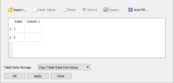
Edit the table header as follows:
Right-click column header
Column 1and select Edit Column Header.The Edit Column Header dialog box appears.
Configure the following settings:
Setting
Value
Name
Speed
Units
rev min^-1
Click OK.
The column header is renamed. You might have to resize the column (drag the column header’s right edge using the mouse) to see the entire label.
Right-click column header
Speed [rev min^-1]and select Insert After.A new column appears, named
Column 2.Right-click column header
Column 2and select Edit Column Header.The Edit Column Header dialog box appears.
Configure the following settings:
Setting
Value
Name
CorrMassFlowRate
Units
kg s^-1
Note that spaces are permitted in column names.
Click OK.
The column header is renamed. Again, you might have to resize the column to see the entire label.
Click Auto Fill.
The Auto Fill Values dialog box appears (replacing the table editor).
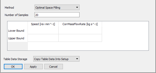
Set Number of Samples to
30.Configure the following settings, clicking once in each cell before typing a value, or clicking twice (but not double-clicking) before pasting a value with Ctrl + v:
Row
Column
Value
Lower Bound
Speed
40000
Upper Bound
Speed
180000
Lower Bound
CorrMassFlowRate
0.01
Upper Bound
CorrMassFlowRate
0.12
Ensure that Table Data Storage is set to
Copy Table Data Into Setup.This will keep the table data with the case instead of writing it to an external (referenced) file. An external file enables other software to update the table data, but creates a need to keep the external file with the case.
Click Apply to close the Auto Fill Values dialog box and return to the table editor.

Note that, as expected, the table is populated with values. The table data is also initialized, and a table function is now listed in the Outline tree view under
Simulation>Expressions, Functions and Variables>User Functions.Note that, if there are values in the table editor at the time you click Auto Fill, the ranges of those values are used to set the corresponding limits in the Auto Fill Values dialog box. If you click OK or Apply in the Auto Fill Values dialog box, automatically generated values replace any existing values in the table editor. You can click Cancel in the Auto Fill Values dialog box to return to the table editor without changing any existing values in the table editor.
Click OK to close the table editor.
Note that, at any time, you could right-click the table function in the Outline tree view and select Edit Table Data to re-invoke the table editor with the table data displayed and ready to edit, export, and so on.
Note also that, had you clicked OK instead of Apply in the Auto Fill Values dialog box, the result would be the same except that you would not be returned to the table editor.
You now have a table function ready to provide input parameters to the case.
In this section, you will define several solution monitors that will result in corresponding operating point output parameters in the simulation results.
Select Insert > Solver > Output Control.
The Output Control details view appears.
On the Monitor tab, under Monitor Points and Expressions, click Add new item
 .
.The Insert Monitor Point dialog box appears.
Set Name to
Isentropic Efficiencyand click OK.Under Monitor Points and Expressions > Isentropic Efficiency:
Set Option to
Expression.Set Expression Value to
Isentropic efficiency.The latter is an expression that is provided with the case.
Click Apply.
Create the following other monitors based on expressions that are provided with the case:
Monitor Name
Expression Value
Mass flow rate
Outlet mass flow rate
Outlet temperature
Outlet Temperature
Total Pressure Ratio
Total pressure ratio
When finished, click OK in the Output Control details view.
An operating point case requires the Operating Points object to be defined in CFX-Pre.
In this object, you can optionally pre-define one or more operating map charts.
Create the Operating Points object and pre-define an operating map chart as follows:
Click Insert > Solver > Operating Points.
The Operating Points details view appears.
Configure the following setting(s):
Tab
Setting
Value
Operating Points
Option
From Table
Table Name
Speeds and Flow Rates
Operating Map Definitions
(Create a new operating map named
PR vs Flow.)Operating Map Definitions
PR vs Flow
> x Variable
CorrMassFlowRate
Operating Map Definitions
PR vs Flow
> y Variable
Total Pressure Ratio
Click OK.
The
Operating Pointsobject appears in the Outline tree view underSimulation Control.
In this section, you will modify the case to make use of the table function data.
In the Outline tree view, edit
Simulation>Flow Analysis 1>R1.Configure the following setting(s):
Tab
Setting
Value
Basic Settings
Domain Models
> Domain Motion
> Angular Velocity
-1*Speeds and Flow Rates.Speed(Index) [a]
Click OK.
Edit
R1 Outlet.Configure the following setting(s):
Tab
Setting
Value
Boundary Details
Mass And Momentum
> Option
Exit Corrected Mass Flow Rate
Mass And Momentum
> Mass Flow Rate
Speeds and Flow Rates.CorrMassFlowRate(Index)
Mass And Momentum
> Mass Flow Rate Area
Total for All Sectors
Click .

Click Solver Control
 .
.Configure the following setting(s):
Tab
Setting
Value
Basic Settings
Convergence Control
> Fluid Timescale Control
> Timescale Control
Physical Timescale
Convergence Control
> Fluid Timescale Control
> Physical Timescale
1 / abs(Speeds and Flow Rates.Speed(Index))
Click .
Click Define Run
 .
.The Write Solver Operating Points Input File dialog box appears (unless the Simulation Control > Execution Control object exists, in which case you can edit that object to plan the name of the solver input file).
Configure the following setting(s):
Setting
Value
File name
Compressor_OM.mdef
Click .
CFX-Solver Manager automatically starts and, on the Define Run dialog box, Solver Input File is set.
Quit CFX-Pre, saving the simulation (
.cfx) file at your discretion.
When CFX-Pre has shut down and the CFX-Solver Manager has started, obtain a solution to the operating point run by following the instructions below.
Ensure that the Define Run dialog box is displayed.
Solver Input File should be set to
Compressor_OM.mdef.On the Operating Points tab, optionally set Concurrency > Option to Maximum Number of Concurrent Jobs and Concurrency > Max. Concurrent Jobs to
2.The allowed number of concurrent jobs depends on license availability.
Note that the Operating Points tab contains other settings that can be used to manage restarts of interrupted runs.
Click Start Run.
CFX-Solver runs and attempts to obtain one solution for each operating point.
The operating point run history page can be seen in the
Operating Point Run Compressor OM 001workspace, on the Run Progress tab. This page includes the current operating point parameter table, which shows the status of each operating point job as well as the input parameters and output parameters. The operating point parameter table also appears in CFD-Post, as will be seen later.The operating point parameter table is essentially the operating point input parameter table (defined in CFX-Pre) with added columns showing output parameter values (each output parameter corresponding to a monitor defined in CFX-Pre). You can export the operating point parameter table by right-clicking a cell and selecting the appropriate command.
Set Workspace to
Operating Point Index 1.You can see residuals and, on the User Points tab, monitor points for the selected operating point job (
Operating Point Index 1).Set Workspace back to
Operating Point Run Compressor OM 001to monitor the overall progress.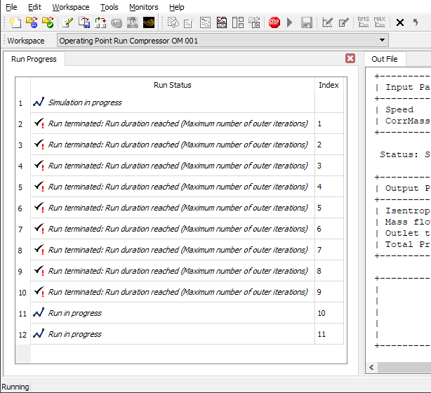
Note that each run is terminated due to reaching the maximum number of outer iterations. The maximum number was set low by design in order to limit the time required to complete this tutorial.
At the end of the run, a dialog box is displayed stating that the simulation has ended.
Select Post-Process Results.
Select Shut down CFX-Solver Manager.
Click .
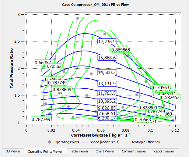
While setting up the case in CFX-Pre, you pre-defined an operating map chart named PR vs Flow with x and y axes of CorrMassFlowRate
and Total Pressure Ratio, respectively.
In this section, you will view that chart, temporarily show response points on it, then add contour lines to it.
Edit
Cases>Compressor_OM_001>Operating Maps>PR vs Flow.The Operating Points Viewer shows the operating point parameter table and the operating map chart that you pre-defined earlier.
As mentioned earlier, the operating point parameter table is essentially the operating point input parameter table (defined in CFX-Pre) with added columns showing output parameter values (each output parameter corresponding to a monitor defined in CFX-Pre). Each row of the table represents an operating point. You can double-click any row in the operating point parameter table to postprocess the 3D results in the same way as for a non-operating-point case (provided that a mesh exists for the selected operating point). Filter settings are available to filter out certain rows of the operating point parameter table. You can export the operating point parameter table from CFD-Post by right-clicking a cell in the table and selecting Export Table Data to CSV.
The operating map chart initially shows the operating points.
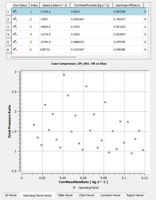
In the details view, on the Chart Data tab, set Chart Data Source > Source Data to
Response Pointsand click Apply.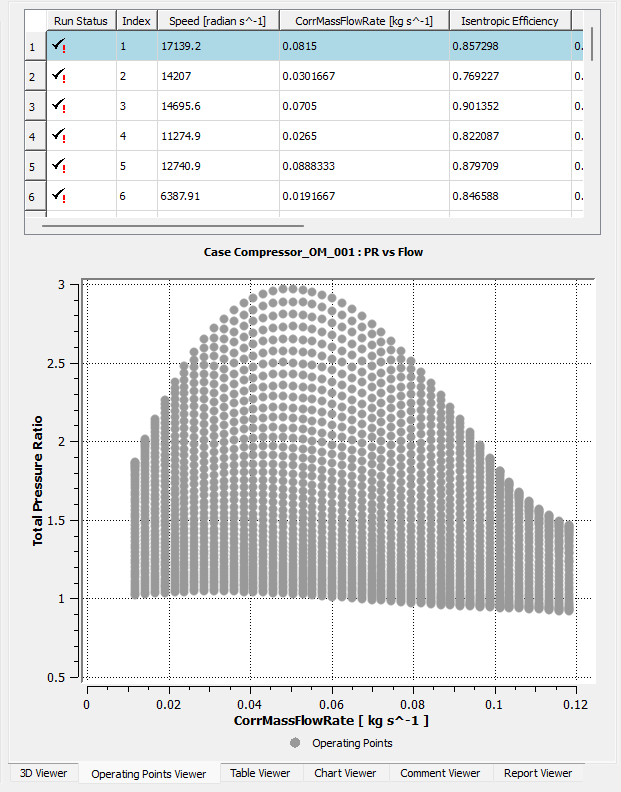
The operating map chart now shows response points, which are sampling points on a response surface (the response surface for
Total Pressure Ratio). The response surface is constructed based on the set of operating points. Using a response surface can yield smoother looking plots. However, it is important to check the quality of the response surface to ensure that the plots that make use of the response surface are not misleading.In the details view, on the Chart Data tab, set Chart Data Source > Source Data to
Operating Pointsand click Apply.In the Outline tree view, edit
Cases>Compressor_OM_001.The details view for the case appears.
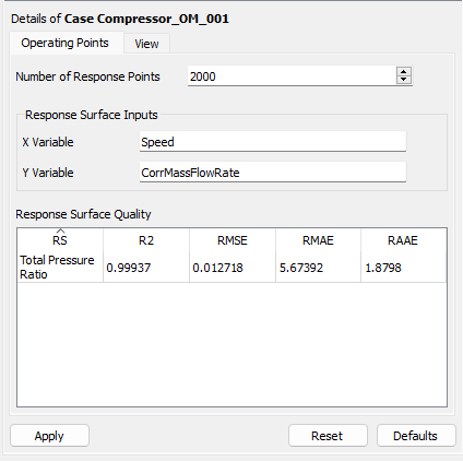
Note that the number of response points sampled from the response surface is adjustable from the Number of Reponse Points setting.
Recall that the input parameters that were defined in the operating point input parameter table in CFX-Pre were
SpeedandCorrMassFlowRate. The table shown in the Operating Points Viewer in CFD-Post (for pre-defined operating map chartPR vs Flow) has columns for those input parameters and additional columns for the output parameters, which came from the solution monitors that you defined earlier. When an operating map chart needs response points for one of those output parameters, a corresponding response surface is generated and quality metrics for that response surface appear as a row in the Reponse Surface Quality table. In this case, there is a row forTotal Pressure Ratiobecause you made an operating map chart that involvedTotal Pressure Ratiosourced from response points. Later in this tutorial, you will examine the quality of theTotal Pressure Ratioresponse surface visually: by plotting contours of constant value on the response surface and overlaying them with operating points.Note that the Reponse Surface Quality table does not list the input parameters, which in this case are
SpeedandCorrMassFlowRate. Response surfaces are not generated for the input parameters.Once again, edit
Cases>Compressor_OM_001>Operating Maps>PR vs Flow.Define a chart series for operating map chart
PR vs Flowto show contours of variableSpeedas follows:Click New
.Settings appear for a new chart series for operating map chart
PR vs Flow.Set Name to
Speed.Leave Type set to
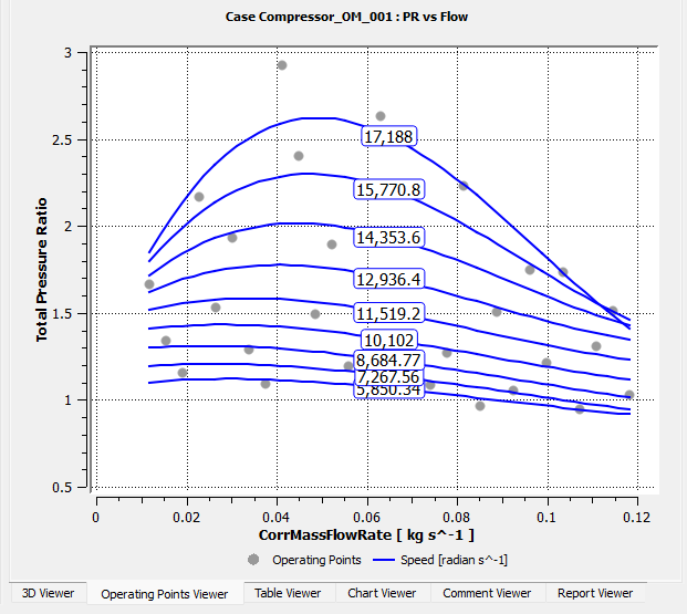
Contour Linesand Parent Series set toOperating Points.Contour lines are always plotted using the same axes as the parent series.
Set Variable to
Speed.Leave Contour Data Source > Source Data set to
Operating Points.Click Apply.
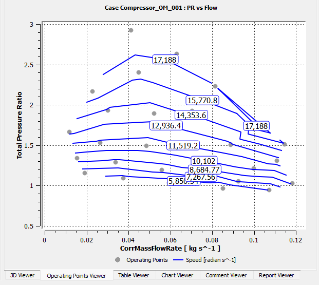
Contours of variable
Speedappear in the operating map chart.Change Contour Data Source > Source Data to
Response Points.Click Apply.
Note how the contours become smoother. They are now created using the response surface for
Total Pressure Ratio.
Using the technique of the previous step, define another chart series to show contours of variable
Isentropic Efficiencybased on, at first, operating points...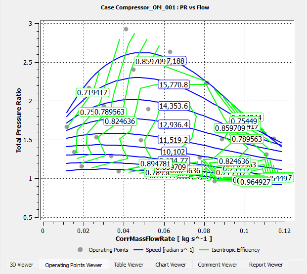
...then response points...
...again, noting the visual difference.
Now that you have defined a plot that uses a response surface for variable
Isentropic Efficiency, a corresponding row exists in the Reponse Surface Quality table.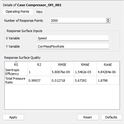
As mentioned earlier, filter settings are available to filter out certain rows of the operating point parameter table. These filter settings also cause operating points to be omitted from the operating map chart and, optionally, all response surfaces that underlie the chart.
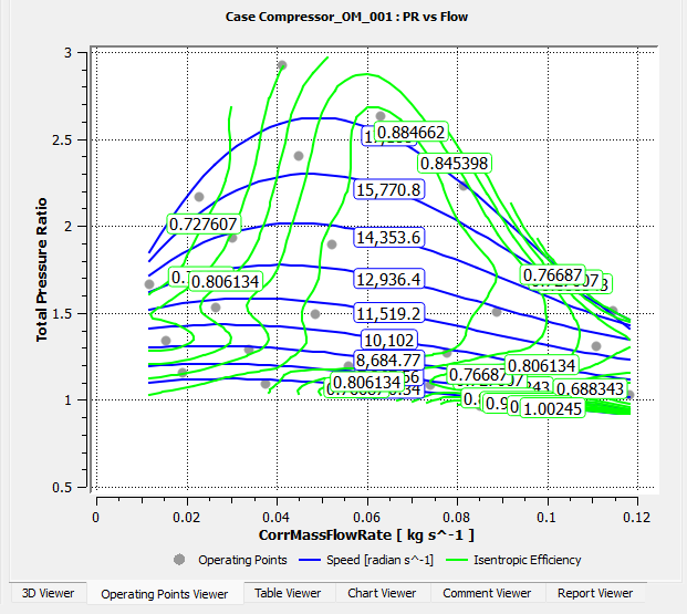
As an exercise, create a filter rule that requires operating points to have a total pressure ratio greater than one in order to be used for the operating map chart or response surfaces.
From the toolbar, click Show operating points filtering controls
 to show the Filter Rules area of the Operating Points Viewer.
Click Add new variable rule
 .
.A new line appears, which looks like the following:

The check box on the left controls whether or not the rule takes effect and the extent of its effect:
A cleared check box (
 )
specifies that the filter rule should be ignored.
)
specifies that the filter rule should be ignored.A partially selected check box (
 )
specifies that all operating points that do not satisfy the filter rule should be excluded
from the operating point parameter table and the operating map chart.
)
specifies that all operating points that do not satisfy the filter rule should be excluded
from the operating point parameter table and the operating map chart.A fully selected check box (
 )
specifies that all operating points that do not satisfy the filter rule should be excluded
from the operating point parameter table, the operating map chart, and the generation of all of
the response surfaces that underlie the operating map chart.
)
specifies that all operating points that do not satisfy the filter rule should be excluded
from the operating point parameter table, the operating map chart, and the generation of all of
the response surfaces that underlie the operating map chart.
Leave the check box fully selected so that the filter rule applies to the operating map chart and its underlying response surfaces.
Set the filter rule to require that the total pressure ratio is greater than one, as shown below.
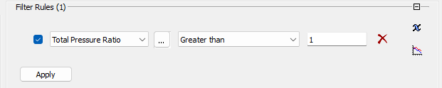
Click Apply.
Some operating points are filtered out; these points are now excluded from the table, the operating map chart, and the response surfaces that underlie the chart.
The operating map chart now appears as follows:
Note that operating maps are included in the Report object.
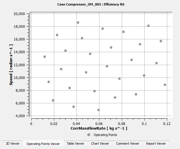
As an exercise, create an operating map chart that can be used to visualize how well the response surface for Total Pressure Ratio
fits the underlying operating point data:
In the Outline tree view, right-click
Cases>Compressor_OM_001>Operating Mapsand select Insert > Operating Map Chart.The Insert CHART dialog box appears.
Set Name to
Efficiency RSand click OK.In the details view, one series is already in the list but requires a definition.
Set Name to
Operating Points.Leave Type set to
Scatter Points.Under Chart Definition, set x Variable and y Variable to
CorrMassFlowRateandSpeed, respectively.These two variables are the operating point input parameters.
Leave Chart Data Source > Source Data set to
Operating Points.Click Apply.
The operating points appear in the operating map chart.
Click New
The details view is ready to define the next series.
Set Name to
TPR - Reponse Surface.Leave Type set to
Contour Lines.Leave Contour Definition > Parent Series set to
Operating Points.Set Variable to
Total Pressure Ratio.Set Contour Data Source > Source Data to
Response Points.Click Apply.
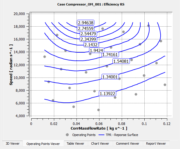
Contours that follow constant values on the response surface for
Total Pressure Ratioappear in the operating map chart.
You can see the operating point values of Total Pressure Ratio by referring to the operating point parameter table.
Ideally, these values should be closely approximated by the response surface.
In general, you can change the quality of a response surface by changing:
The number of operating points,
The input parameter values for existing operating points,
Filter rules that affect the response surfaces (due to having a fully selected check box), and
The number of response points.
The key to a good response surface is a good distribution of input parameters.