


A single-stage turbomachinery configuration with pitch change can be modeled using the Fourier Transformation method. This method is particularly useful for modeling a large-pitch-change configuration and when it is not possible to use the Time Transformation method.
This tutorial includes:
- 35.1. Tutorial Features
- 35.2. Overview of the Problem to Solve
- 35.3. Preparing the Working Directory
- 35.4. Defining and Obtaining a Solution for the Time Integration Solution Method Case
- 35.5. Defining and Obtaining a Solution for the Harmonic Balance Solution Method Case
- 35.6. Postprocessing the Transient Rotor-stator Solution
Important: This tutorial requires file TimeBladeRowIni_001.res, which is produced by following tutorial Time Transformation Method for a Transient Rotor-stator Case.
In this tutorial you will learn about:
Component | Feature | Details |
|---|---|---|
CFX-Pre | User Mode | Turbo Wizard |
General mode | ||
|
Analysis Type |
Transient Blade Row | |
|
Fourier Transformation Pitch Change Model | ||
|
Time Integration Solution Method | ||
|
Harmonic Balance Solution Method | ||
Fluid Type | Air Ideal Gas | |
Domain Type | Multiple Domains | |
Rotating Frame of Reference | ||
Turbulence Model | Shear Stress Transport | |
Heat Transfer | Total Energy | |
Boundary Conditions | Inlet (Subsonic) | |
Outlet (Subsonic) | ||
Wall (Counter Rotating) | ||
CFD-Post | Plots | Vector |
Contour | ||
Data Instancing | ||
Time Chart | ||
Animation |
The goal of this tutorial is to set up a transient blade row calculation using the Fourier Transformation model. It uses an axial turbine to illustrate the basic concepts of setting up, running, and monitoring a transient blade row problem in Ansys CFX. It also describes the postprocessing of transient blade row results using the tools provided in CFD-Post for this type of calculation.
The full geometry of the axial rotor-stator stage selected for modeling contains 36 stator blades and 42 rotor blades.
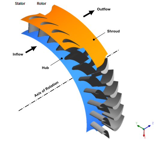
The geometry to be modeled consists of a pair of rotor blade passages and a pair of stator blade passages. Pairs of passages are needed because the Fourier Transformation method uses a double-passage strategy. Each rotor blade passage is an 8.571° section (360°/42 blades), while each stator blade passage is a 10° section (360°/36 blades). The pitch ratio at the interface between the pair of rotor passages and the pair of stator passages is 0.8571 (that is, 6/7).
You should always try to obtain a pitch ratio as close to 1 as possible in your model to minimize approximations, but this must be weighed against computational resources. A full machine analysis (modeling all rotor and stator blades) eliminates pitch change, but requires significant computational time. For this rotor-stator geometry, a 1/6 machine section (7 rotor blades, 6 stator blades) would produce a pitch ratio of 1.0, but this would require a model about 3 times larger than in this tutorial example.
In this example, the rotor rotates about the Z axis at 3500 rev/min (positive rotation following the right hand rule) while the stator is stationary. Rotational periodicity boundaries with phase lag are used to enable only a small section of the full geometry to be modeled.
The flow is modeled as being turbulent and compressible. Profile boundary conditions are used at the inlet and outlet. In this tutorial, the profiles are a function of radial coordinate only. These profiles were obtained from previous simulations of the upstream and downstream stages.
The following steps outline the overall approach:
Define the transient blade row simulation using the Turbomachinery wizard in CFX-Pre.
Import the stator and rotor meshes, which were created in Ansys TurboGrid.
Enter the basic model definition.
Set the profile boundary conditions using CFX-Pre in General mode.
Run the transient blade row simulation using the steady-state results from Time Transformation Method for a Transient Rotor-stator Case as an initial guess.
Create a working directory.
Ansys CFX uses a working directory as the default location for loading and saving files for a particular session or project.
Download the
fourier_blade_row.zipfile here .Unzip
fourier_blade_row.zipto your working directory.Ensure that the following tutorial input files are in your working directory:
TBRInletProfile.csvTBROutletProfile.csvTBRTurbineRotor.gtmTBRTurbineStator.gtmTimeBladeRowIni_001.res(produced by following tutorial Time Transformation Method for a Transient Rotor-stator Case)
Set the working directory and start CFX-Pre.
For details, see Setting the Working Directory and Starting Ansys CFX in Stand-alone Mode.
This tutorial uses the Turbomachinery wizard in CFX-Pre. This preprocessing mode is designed to simplify the setup of turbomachinery simulations.
In CFX-Pre, select > .
Select Turbomachinery and click .
Select > .
Under File name, type
FourierBladeRowTime.Click .
If you are notified that the file already exists, click .
In the Basic Settings panel, configure the following settings:
Setting
Value
Machine Type
Axial Turbine
Axes
> Coordinate Frame
Coord 0
Axes
> Rotation Axis
Z
Analysis Type
> Type
Transient Blade Row
Analysis Type
> Method
Fourier Transformation
Click Next.
The Fourier Transformation method requires two rotor blade passages and two stator blade passages. You will define two new components and import their respective meshes.
Right-click in the blank area and select Add Component from the shortcut menu.
Create a new component of type
StationarynamedS1and click .Configure the following setting(s):
Setting
Value
Mesh
> File
TBRTurbineStator.gtm [a]
Expand the Passage and Alignment section and click Edit.
Configure the following setting(s):
Setting
Value
Passage and Alignment
> Passages to Model
2
After clicking Done, you will see that the stator blade passage is correctly replicated and the resulting mesh contains two stator blade passages as required by the Fourier Transformation model. This also creates the Sampling Interface (S1 Internal Interface 1).
Right-click in the blank area and select Add Component from the shortcut menu.
Create a new component of type
Rotating, namedR1and click .Configure the following setting(s):
Setting
Value
Component Type
> Value
3500 [rev min^-1] [a]
Mesh
> File
TBRTurbineRotor.gtm
Expand the Passage and Alignment section and click Edit.
Configure the following setting(s):
Setting
Value
Passage and Alignment
> Passages to Model
2
After clicking Done, you will see that the rotor blade passage is correctly replicated and the resulting mesh contains two rotor blade passages as required by the Fourier Transformation model. This also creates the Sampling Interface (R1 Internal Interface 1).
Click Next.
In this section, you will set properties of the fluid domain and some solver parameters.
Configure the following setting(s):
Setting
Value
Fluid
Air Ideal Gas
Model Data
> Reference Pressure
0 [atm] [a]
Model Data
> Heat Transfer
Total Energy
Model Data
> Turbulence
Shear Stress Transport
Inflow/Outflow Boundary Templates
> P-Total Inlet P-Static Outlet
(Selected)
Inflow/Outflow Boundary Templates
> Inflow
> P-Total
169000 [Pa] [b]
Inflow/Outflow Boundary Templates
> Inflow
> T-Total
306 [K] [b]
Inflow/Outflow Boundary Templates
> Inflow
> Flow Direction
Normal to Boundary
Inflow/Outflow Boundary Templates
> Outflow
> P-Static
110000 [Pa] [b]
Interface
> Default Type
Transient Rotor Stator
Click Next.
Under the Interface Definition section, you can observe that both the Fourier coefficient sampling interfaces S1 Internal Interface 1 and R1 Internal Interface 1, as well as, the Phase-shifted interfaces S1 to S1 Periodic 1 and R1 to R1 Periodic 1 are automatically created.
Click Next.
In this section, you will specify the type of disturbance being imposed.
Configure the following setting(s):
Setting
Value
Disturbance
> Fourier Transformation
> Type
Rotor Stator
Disturbance
> Fourier Transformation
> Domain Interface
R1 to S1
Continue to click Next until you reach
Final Operations.Set Operation to
Enter
General Mode
because you will continue to define the simulation through settings not available in the Turbomachinery wizard.Click Finish.
Verify the following settings, which affect the accuracy of the simulation:
Edit
R1.Configure the following setting(s):
Tab
Setting
Value
Basic Settings
Domain Models
> Domain Motion
> Alternate Rotation Model
(Selected)
Fluid Models
Heat Transfer
> Incl. Viscous Work Term
(Selected)
Click .
The inlet and outlet boundary conditions are defined using profiles in your working directory. Boundary profile data must be initialized before they can be used for boundary conditions.
Select Tools > Initialize Profile Data.
The Initialize Profile Data dialog box appears.
Beside Profile Data File, click Browse
 .
.The Select Profile Data File dialog box appears.
From your working directory, select
TBRInletProfile.csv.Click .
Click .
The profile data is read into memory.
Under Data File, click Browse
.From your working directory, select
TBROutletProfile.csv.Click .
Click .
Note: After profile data has been initialized from a file, the profile data file should not be deleted or otherwise removed from its directory. By default, the full file path to the profile data file is stored in CFX-Pre, and the profile data file is read directly by CFX-Solver each time the solver is started or restarted.
Edit
S1 Inlet.Configure the following setting(s):
Tab
Setting
Value
Basic Settings
Profile Boundary Conditions
> Use Profile Data
(Selected)
Profile Boundary Setup
> Profile Name
inlet
Click Generate Values.
This causes the profile values of
Total PressureandTotal Temperatureto be applied at the nodes on the inlet boundary. It also causes entries to be made in the Boundary Details tab. In order to later reset the velocity values at the main inlet to match those that were originally read from the profile data file, revisit the Basic Settings tab for this boundary and click Generate Values.Configure the following setting(s):
Tab
Setting
Value
Boundary Details
Mass and Momentum
> Option
Total Pressure (stable)
Mass and Momentum
> Relative Pressure
inlet.Total Pressure(r)
Flow Direction
> Option
Cylindrical Components
Flow Direction
> Axial Component
1
Flow Direction
> Radial Component
0
Flow Direction
> Theta Component
0
Heat Transfer
> Option
Total Temperature
Heat Transfer
> Total Temperature
inlet.Total Temperature(r)
Click .
Edit
R1 Outlet.Configure the following setting(s):
Tab
Setting
Value
Basic Settings
Frame Type
Rotating
Profile Boundary Conditions
> Use Profile Data
(Selected)
Profile Boundary Setup
> Profile Name
outlet
Click Generate Values.
Configure the following setting(s):
Tab
Setting
Value
Boundary Details
Mass and Momentum
> Option
Static Pressure
Mass and Momentum
> Relative Pressure
outlet.Pressure(r)
Click .
You will set the simulation to be solved using the Fourier Transformation method.
Edit
Transient Blade Row Models.Configure the following setting(s):
Setting
Value
Transient Method
> Time Period
> Option
Automatic
Transient Method
> Time Steps
> Option
Timestep Multiplier
Transient Method
> Time Steps
> Timestep Multiplier
5
Transient Method
> Time Duration
> Option
Number of Periods per Run
Transient Method
> Time Duration
> Periods per Run
20
Note:The passing period is automatically calculated as: 2 * pi / (Number of Blades * Angular Velocity). The Passing Period setting cannot be edited.
The number of time steps per period should always be larger than 2 * Number of Fourier Coefficients + 1 to be used for postprocessing. When the time step size is set using the
Timestep Multiplieroption, the number of time steps per period is the product of the values of Min Timesteps / Per. and Timestep Multiplier.The time step size is also automatically calculated as: Passing Period / Number of Time Steps per Period. The Timestep setting cannot be edited.
Click .
For transient blade row calculations, a minimal set of variables
are selected to be computed using Fourier coefficients. It is convenient
to postprocess variables in the stationary frame when multiple frames
of reference are present. Here, you will add the Velocity
in Stn Frame and Mach Number in Stn Frame variables to the default list.
In addition, monitor points can be used to effectively compare the Fourier Transformation results against a reference case. They provide useful information on the quality of the reference phase and frequency produced in the simulation. As the simulation converges, the user points should display a periodic pattern.
Note:
When comparing to a reference case, make sure monitor points are placed in the same relative locations with respect to the initial configuration in both cases.
It is important to check that the solver equations are being solved correctly. Monitoring pressure provides feedback on the momentum equations while monitoring temperature provides feedback on the energy equations.
For diagnostic purposes, you should have several monitor points. Here, two monitor points will be used for demonstration purposes.
Set up the output control and create monitor points as follows:
Click Output Control
 .
.Click the Trn Results tab.
Configure the following setting(s):
Setting
Value
Transient Blade Row Results
> Extra Output Variables List
(Selected)
Transient Blade Row Results
> Extra Output Variables List
> Extra Output Var. List
Velocity in Stn Frame, Mach Number in Stn Frame[a]
Click the Monitor tab.
Configure the following setting(s):
Setting
Value
Monitor Objects
(Selected)
Monitor Objects
> Efficiency Output
(Cleared)
Create a monitor point named
rotor_P1.Under Monitor Objects > Monitor Points and Expressions > rotor_P1, configure the following settings:
Setting
Value
Option
Cylindrical Coordinates
Output Variables List
Pressure, Temperature, Total Pressure, Total Temperature, Velocity
Position Axial Comp.
0.211 [m]
Position Radial Comp.
0.2755 [m]
Position Theta Comp.
182 [degree]
Create an additional monitor point named
stator_P1.Under Monitor Objects > Monitor Points and Expressions > stator_P1, configure the following settings:
Setting
Value
Option
Cylindrical Coordinates
Output Variables List
Pressure, Temperature, Total Pressure, Total Temperature, Velocity
Position Axial Comp.
0.202 [m]
Position Radial Comp.
0.2755 [m]
Position Theta Comp.
178 [degree]
Click .
Save the simulation.

Here you will prepare the case for execution and initialize the solution with steady-state results. Instead of obtaining steady-state results by setting up and running the steady-state solution for this case, which has a double passage configuration, you will import a results file from another steady-state simulation, which happens to have a single passage (see Defining a Steady-state Case in CFX-Pre). Because that other simulation involves only a single passage, you will use replication control settings to apply those results to both passages in this simulation.
In the Outline tree view, right-click
Simulation Controland select Insert > Execution Control.Configure the following setting(s):
Tab
Setting
Value
Run Definition
Run Settings
> Double Precision
(Selected)
Initial Values
Initial Values Specification
(Selected)
Initial Values Specification
> Initial Values
Initial Values 1
Initial Values Specification
> Initial Values
> Initial Values 1
> File Name
TimeBladeRowIni_001.res [a]
Initial Values Specification
> Initial Values Control
(Selected)
Initial Values Specification
> Initial Values Control
> Continue History From
(Selected)
On the Initial Values tab, create an interpolation mapping item named
R1 Interpolation.Under Initial Values Specification > Initial Values > Initial Values 1 > Interpolation Mapping > R1 Interpolation, configure the following settings:
Setting
Value
Source Location
R1
Target Location
R1
Replication Control
(Selected)
Replication Control
> Passages in 360
42
Replication Control
> Total Num. Instances
2
Create a second interpolation mapping item named
S1 Interpolation.Under Initial Values Specification > Initial Values > Initial Values 1 > Interpolation Mapping > S1 Interpolation, configure the following settings:
Setting
Value
Source Location
S1
Target Location
S1
Replication Control
(Selected)
Replication Control
> Passages in 360
36
Replication Control
> Total Num. Instances
2
Click .
Click Define Run
 .
.The CFX-Solver input file
FourierBladeRowTime.defis created by default.CFX-Solver Manager automatically starts and, on the Define Run dialog box, the Solver Input File is set.
If using stand-alone mode, quit CFX-Pre, saving the simulation (
.cfx) file at your discretion.
At this point, CFX-Pre has been shut down, and the Define Run dialog box is displayed in CFX-Solver Manager. The initial values file has already been specified (see Setting the Execution Control). You will now obtain a solution to the CFD problem.
Click .
CFX-Solver runs and attempts to obtain a solution. This can take a long time depending on your system. Eventually a dialog box is displayed.
Note:Before the simulation begins, the "Transient Blade Row Post-processing Information" summary in the CFX-Solver Output file will display the time step range over which the solver will accumulate the Fourier coefficients.
During the run, the "Fourier Transformation Information" summary in the CFX-Solver Output file displays the time step at which the full Fourier Transformation Model is activated.
Monitor points of similar values can be grouped together by right-clicking to the right of the User Points tab, selecting New Monitor, and clicking . In the New Monitor dialog box, you can name the new monitor point and select the variables to monitor in the Monitor Properties dialog box.
After the simulation has proceeded for some time, observe the periodic nature of the monitor point values.
When CFX-Solver is finished, clear the check box next to Post-Process Results.
Click .
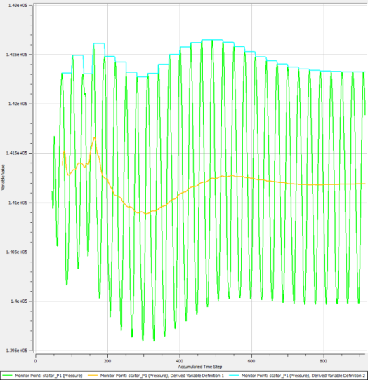
If you did not observe periodic monitor behavior within 20 passing periods of the stator, you should create statistical derived variables to verify that the solution approaches periodicity by following the procedure below:
Select Workspace > New Monitor.
Change the name to
Stator Pressure.Click .
The Monitor Properties dialog box appears.
On the Plot Lines tab, select
USER POINTS>Pressure>stator_P1.Click Apply.
A plot line of pressure (in Pa) at
stator_P1versus accumulated time step appears.Click the Derived Variables tab.
Create a derived variable named
Avg Over Passing Period.The Derived Variable Properties dialog box appears.
Configure the following setting(s):
Setting
Value
Statistics
> Statistics Type
Arithmetic Average
Statistics
> Interval Option
Moving Interval
Statistics
> Interval Definition
> Option
Timesteps
Statistics
> Interval Definition
> Number of Timesteps
30
Click OK.
Return to the Monitor Properties dialog box.
In the Workspace Derived Variables list box, select
Avg Over Passing Period.Click Apply.
A plot line of the average pressure at
stator_P1over a moving passing period appears.Create a derived variable named
Max Over Passing Period.The Derived Variable Properties dialog box appears.
Configure the following setting(s):
Setting
Value
Statistics
> Statistics Type
Maximum
Statistics
> Interval Option
Moving Interval
Statistics
> Interval Definition
> Option
Timesteps
Statistics
> Interval Definition
> Number of Timesteps
30
Click OK.
Return to the Monitor Properties dialog box.
In the Workspace Derived Variables list box, select
Max Over Passing Period.Click OK.
A plot line of the maximum pressure at
stator_P1over a moving passing period appears.
Both derived variable plot lines should appear to approach stable values. If you had set the simulation to run for 25 passing periods, the plot monitor would resemble the image below:
In this part of the tutorial, you will modify the Time Integration solution method case that was set up in the previous part of the tutorial in order to use the Harmonic Balance solution method. As in the previous part, the result from the steady-state simulation is used as an initial guess to speed convergence.
This step involves opening the Time Integration simulation and saving it to a different location.
Ensure that the following tutorial input files are in your working directory:
FourierBladeRowTime.cfxTimeBladeRowIni_001.res
Set the working directory and start CFX-Pre if it is not already running.
For details, see Setting the Working Directory and Starting Ansys CFX in Stand-alone Mode.
If the Time Integration simulation is not already opened, then open
FourierBladeRowTime.cfx.Save the case as
FourierBladeRowHarmonic.cfxin your working directory.
There are many common steps between setting up Time Integration and Harmonic Balance Transient Rotor-stator cases, including using the same Fourier Transformation pitch change model. Here, only the differences are highlighted.
In this section, you will change the transient method to Harmonic
Balance.
In the Outline tree view, edit
Flow Analysis 1>Transient Blade Row Models.Configure the following setting(s):
Tab
Setting
Value
Basic Settings
Transient Method
> Option
Harmonic
    Balance
Transient Method
> Number of Modes
3
Note that, in the Transient Blade Row Models details view, on the Basic Settings tab, the settings for Time Period, Time Steps and Time Duration have disappeared.
Click OK.
There is no need to specify the period involved when selecting Harmonic Balance in combination with the Fourier Transformation model.
The period in each domain is obtained by the blade passing frequency, which is proportional to the blade count in the adjacent row.
Click Solver Control
 .
.Configure the following setting(s):
Tab
Setting
Value
Basic Settings
Transient Scheme
> Option
Harmonic Balance
Convergence Control
> Min. Iterations
1
Convergence Control
> Max. Iterations
200
Convergence Control
> Fluid Timescale Control
> Timescale Control
Physical Timescale
Convergence Control
> Fluid Timescale Control
> Physical Timescale
((1 [rev] / 42) / 3500 [rev min^-1]) / 20
Click OK.
The physical timescale is usually set as a fraction of the smallest time period involved. In this case 1/20th of the rotor blade passing period is used as the physical timescale. A larger physical timescale speeds convergence but can lower stability. In general, if the solution becomes unstable or does not converge, you should use a smaller fraction when computing the physical timescale.
In preparation for a Harmonic Forced Response analysis during postprocessing, you will set CFX-Pre to export a harmonic of the pressure on the rotor’s surface.
In order to do this, you will indicate the frequency of excitation of the rotor by specifying an engine order value, which represents the number of disturbances (or pulses) per revolution of the engine.
In this case, any given rotor blade is excited by 36 disturbances per engine revolution: one disturbance from each of the 36 stator blades.
Click Output Control
.Click the Export tab.
Under Export Results, click Add new item
 .
.The Insert Export Results dialog box appears.
Accept the default name by clicking .
Under Export Results > Export Results 1 > Export Format, ensure that Option is set to
CFX CSV BC Profileand select Include Topology.When selected, the Include Topology setting causes connectivity data to be included so that the resulting surface data can be used as a locator in CFD-Post, for example for a contour plot.
Under Export Results > Export Results 1 > Export Surface, click Add new item
.The Insert Export Surface dialog box appears.
Accept the default name by clicking .
Configure the following settings under Export Results > Export Results 1 > Export Surface > Export Surface 1:
Setting
Value
Option
Harmonic Forced Response
Location Type
> Option
BoundaryLocation Type
> Boundary
R1 Blade
Excitation Frequency
> Option
Engine Order
Excitation Frequency
> Engine Order
36
Click OK.
Later in this tutorial, when the CFX-Solver has finished its calculations, the solver will write
file ExportResults1_<a number>.csv where ExportResults1
is the given name of the surface (under "[Name]", as shown below) and
<a number> is the applicable outer loop iteration number (padded with leading
zeros to make 6 digits).
After the exported file is written, its contents will look similar to the following:
[Name]
Export Surface 1

[Parameters]
Ncompt = 1
Nnodes = 3680
Rotation Axis From = 0.0000000 [m], 0.0000000 [m], 0.0000000 [m]
Rotation Axis To   = 0.0000000 [m], 0.0000000 [m], 1.0000000 [m]
Rotating Speed     = 366.51914 [s^-1 rad]
Frequency          = 2100.0000 [Hz]
Engine Order       = 36

[Spatial Fields]
x, y, z

[Data]
x [ m ], y [ m ], z [ m ], Real Pressure [ kg m^-1 s^-2 ], Imaginary Pressure [ kg m^-1 s^-2 ], Node Number
-2.44994841E-001,  1.58908837E-003,  2.15076035E-001, -5.99750474E+001, -1.75136536E+002,         0
-2.45487356E-001,  1.59036453E-003,  2.15079039E-001, -7.26132011E+001, -2.26077478E+002,         1
-2.46203489E-001,  1.59221122E-003,  2.15083406E-001, -1.52475786E+002, -1.82970865E+002,         2
-2.47237201E-001,  1.59486280E-003,  2.15089716E-001, -2.65408934E+002, -3.06071903E+001,         3
-2.48715507E-001,  1.59862583E-003,  2.15098751E-001, -2.95003528E+002,  5.97159931E+001,         4
-2.50804203E-001,  1.60388403E-003,  2.15111541E-001, -2.81566347E+002,  1.12160789E+002,         5
.
.
.
-2.97890454E-001, -3.19597847E-002,  2.58500217E-001, -4.62603071E+001, -1.13633158E+002,      3675
-2.97474064E-001, -3.56276826E-002,  2.57683679E-001, -2.49212458E+001, -1.51912000E+001,      3676
-2.97497251E-001, -3.54335493E-002,  2.57406431E-001, -2.59207308E+001, -2.29944420E+001,      3677
-2.97524623E-001, -3.52029722E-002,  2.57077487E-001, -2.78774687E+001, -3.31765348E+001,      3678
-2.97558085E-001, -3.49189960E-002,  2.56672866E-001, -2.92674110E+001, -4.02254086E+001,      3679

[Faces]
       148,       147,      1260,      1261
      1261,      1260,        84,        85
       149,       148,      1261,      1262
      1262,      1261,        85,        86
       150,       149,      1262,      1263
      1263,      1262,        86,        87
       151,       150,      1263,      1264
      1264,      1263,        87,        88
.
.
.
Note that the connectivity data consists of the Node Number data column and the [Faces] section.
Click Execution Control
 .
.Configure the following setting(s):
Tab
Setting
Value
Run Definition
Input File Settings
> Solver Input File
FourierBladeRowHarmonic.def [a]
Confirm that the rest of the execution control settings are set appropriately.
Click .
Click Define Run
.The CFX-Solver input file
FourierBladeRowHarmonic.defis created by default.CFX-Solver Manager automatically starts and, on the Define Run dialog box, the Solver Input File is set.
If using stand-alone mode, quit CFX-Pre, saving the simulation (
.cfx) file at your discretion.
At this point, CFX-Pre has been shut down, and the Define Run dialog box is displayed in CFX-Solver Manager. The initial values file has already been specified (see Setting the Execution Control). You will now obtain a solution to the CFD problem.
Click .
CFX-Solver runs and attempts to obtain a solution. This can take a long time depending on your system. Eventually a dialog box is displayed.
When CFX-Solver is finished, clear the check box next to Post-Process Results.
Click .
The postprocessing steps outlined here can be equally used on either of the Transient Rotor-stator solutions obtained in Defining and Obtaining a Solution for the Time Integration Solution Method Case and Defining and Obtaining a Solution for the Harmonic Balance Solution Method Case. The results should be similar and the differences between the two will be minimized by comparing a time-resolved transient case to a modal-resolved harmonic balance case (that is, a case where increasing the number of modes or time planes does not result in solution change).
In a transient blade row run, flow field variables are compressed using the Fourier coefficient method. These variables are accumulated at the end of the simulation. This enables you to navigate through any time instance, within the common period, without having to load multiple transient results files. By default CFD-Post displays results corresponding to the end the simulation.
To get started, follow these steps:
Start CFD-Post and load results from either FourierBladeRowTime_001.res or FourierBladeRowHarmonic_001.res.
When CFD-Post opens, if you see the Domain Selector dialog box, ensure that all the domains are selected, then click to load the results from these domains.
If you see a message regarding transient blade row postprocessing, click .
Create a turbo surface to be used for making plots:
Click the Turbo tab.
If you see the Turbo Initialization dialog box, click , otherwise click the button, which is visible initially by default, or after double-clicking the Initialization object in the Turbo tree view.
Select Insert > Location > Turbo Surface.
Change the name to
Span 50.Configure the following setting(s):
Tab
Setting
Value
Geometry
Definition
> Method
Constant Span
Definition
> Value
0.5
Click .
Turn off the visibility of
Span 50by clearing its check box in the Outline tree view.
Click Insert > Vector and accept the default name.
Configure the following setting(s):
Tab
Setting
Value
Geometry
Definition
> Locations
Span 50
Definition
> Variable
Velocity in Stn Frame
Click .
The vector plot shows
Velocity in Stn Framevalues corresponding to the end of a common period.Now you will align the rotor with the stator, as it was in the solver input file.
Click Timestep Selector
 .
.Select the 1st time step.
Click to load the time step, and then click Close to exit the dialog box.
The rotor blades move to their starting positions.
Turn off the visibility of
Vector 1.Click Insert > Contour and accept the default name.
Configure the following setting(s):
Tab
Setting
Value
Geometry
Locations
Span 50
Variable
Pressure
Range
Local
# of Contours
21
Click .
The contour plot shows Pressure values
corresponding to the specified time step.
In this section, you will compute and plot the magnitude of the forces that the flow applies on the rotor blade. For a transient blade row case, CFD-Post automatically reconstructs variables for the flow solution time based on the last time step. Intermediate time steps for time instances in the common period are located in the Timestep Selector.
For the time integration solution method case, you set 35 time steps per stator blade passing period in Setting up a Transient Blade Row Model. Because there are six stator blade passing periods in a common period, the total number of intermediate time steps in the common period is 210. Because the solver has reconstructed results over four common periods, there are 840 time steps. If you are currently postprocessing the time integration solution method case, reduce the total number of time steps over four periods from 840 to 280, as follows, to speed generation of the time chart:
Click Timestep Selector
.Configure the following setting(s):
Tab
Setting
Value
Timestep Selector
Timestep Sampling
Uniform
Number of Timesteps
70
Click .
The Timestep Selector now shows a total of 280 steps over four common periods (shown under the Phase column).
Compute the net force on the pair of rotor blades in the rotor domain (that is, the net force on region R1 Blade):
Select Insert > Expression.
In the Insert Expression dialog box, type
forces on rotor blades.Click .
Set Definition to
sqrt(force_x()@
R1 Blade ^2 + force_y()@ R1 Blade ^2 + force_z()@ R1 Blade ^2)
Click to create the expression.
Create a transient chart showing force:
Select Insert > Chart and accept the default name.
Configure the following setting(s):
Tab
Setting
Value
General
XY - Transient or Sequence
(Selected)
Data Series
Series 1
> Data Source
> Expression
(Selected)
Series 1
> Data Source
> Expression
forces on rotor blades
If you are postprocessing the time integration solution method case, configure the following settings to plot only the last common period:
Tab
Setting
Value
X Axis
Axis Range
> Determine ranges automatically
(Cleared)
Axis Range
> Min
0.00857143
Axis Range
> Max
0.0114286
Click .
The chart displayed in the Chart Viewer shows the net force on the modeled pair of rotor blades as a function of time.
Select File > Import > Import Surface, Line or Point Data.
The Import Surface, Line or Point Data dialog box appears.
Click Browse
.Select the Export Results (.csv) file from the run directory for the Harmonic Analysis: FourierBladeRowHarmonic_001.
Click Open.
In the Import Surface, Line or Point Data dialog box, ensure that Import As is set to
Surface or Line.Click OK.
The surface appears in the 3D Viewer.
You can use the surface as a locator for a contour plot of Real Pressure or Imaginary Pressure.
Data instancing uses Fourier interpolation to reproduce other passages that are not included in a simulation. In this section, you will use data instancing to replicate enough passages in the rotor and stator domains to recover unity pitch ratio across the rotor-stator interface.
From the Outline tree view, edit
R1.In the Data Instancing tab, set Number of Data Instances to 7.
Click .
On the 3D Viewer tab, CFD-Post displays 14 rotor blades.
From the Outline tree view, edit
S1.In the Data Instancing tab, set Number of Data Instances to 6.
Click .
On the 3D Viewer tab, CFD-Post displays 12 stator blades.
CFD-Post now computes forces on rotor blades on all 14 blade instances in R1 Blade. However, Chart 1 will not reflect this change automatically. To
update Chart 1:
At the top of the Chart Viewer, click the Refresh button.
In this section, you will use graphical instancing to visually complete the full wheel. You will make copies of the wheel segment that was completed using data instancing.
From the Outline tree view, turn off the visibility of
Wireframe.Edit
R1.Configure the following setting(s):
Tab
Setting
Value
Instancing
Number of Graphical Instances
3
Instance Definition
Custom
Passages per Component
14
Click .
Edit
S1.Configure the following setting(s):
Tab
Setting
Value
Instancing
Number of Graphical Instances
3
Instance Definition
Custom
Passages per Component
12
Click .
The Graphics Instancing feature makes graphical copies of objects and places them at an angular position computed using the Number of Passages and Number of Passages per Component on the Instancing panel. To complete the full wheel, you replicated the 1/3 wheel sector, which was obtained using data instancing, three times. On the 3D Viewer tab, CFD-Post displays the pressure plot on
Span 50over the full wheel.
With the Timestep Selector set to time
step 0, you will make an animation showing the
relative motion starting from this time step and lasting for one stator
blade passing period.
Click the 3D Viewer tab.
Position the geometry for the animation by right-clicking on a blank area in the viewer and selecting Predefined Camera > View From -X.
Click Animation
 .
.The Animation dialog box appears.
Set Type to Keyframe Animation.
Click New
to create KeyframeNo1.Select
KeyframeNo1, then set # of Frames to70, then press Enter while in the # of Frames box.Tip: Be sure to press Enter and confirm that the new number appears in the list before continuing.
This will place 70 intermediate frames between the keyframes, for a total of 72 frames.
Use the Timestep Selector to load time step
70and then close the dialog box.In the Animation dialog box, click New to create
KeyframeNo2.Click More Animation Options
 to expand the Animation dialog
box.
to expand the Animation dialog
box.Select Save Movie.
Specify a filename for the movie.
Set Format to
MPEG1.Click To Beginning
 to rewind the active keyframe to
 KeyframeNo1.Note: The active keyframe is indicated by the value appearing in the F: field in the middle of the Animation dialog box. In this case it will be
1.Wait for CFD-Post to finish loading the objects for this frame before proceeding.
Click Save animation state
 and save the animation to a file. This will enable
you to quickly restore the animation in case you want to make changes.
Animations are not restored by loading ordinary state files (those
with the
and save the animation to a file. This will enable
you to quickly restore the animation in case you want to make changes.
Animations are not restored by loading ordinary state files (those
with the .cstextension).Click Play the animation
 .
.Note: It takes a while for the animation to be completed. To view the movie file, you will need to use a media player that supports the MPEG format.
From the animation and plots, you will see that the flow is continuous across the interface. This is because CFD-Post is capable of interpolating the flow field variables to the correct time and position using the computed Fourier coefficients.
When you have finished, close the Animation dialog box and then close CFD-Post, saving the animation state at your discretion.