


This tutorial includes:
In this tutorial you will learn about:
Using the Turbo Wizard in CFX-Pre to quickly specify a turbomachinery application.
Multiple Frames of Reference and Generalized Grid Interface.
Using a Frozen Rotor interface between the rotor and stator domains.
Modifying an existing simulation.
Setting up a transient calculation.
Using a Transient Rotor-Stator interface condition to replace a Frozen Rotor interface.
Creating a transient animation showing domain movement in CFD-Post.
|
Component |
Feature |
Details |
|---|---|---|
|
CFX-Pre |
User Mode |
Turbo Wizard |
|
Analysis Type |
Steady State | |
|
Transient | ||
|
Fluid Type |
Ideal Gas | |
|
Domain Type |
Multiple Domain | |
|
Rotating Frame of Reference | ||
|
Turbulence Model |
k-Epsilon | |
|
Heat Transfer |
Total Energy | |
|
Boundary Conditions |
Inlet (Subsonic) | |
|
Outlet (Subsonic) | ||
|
Wall: No-Slip | ||
|
Wall: Adiabatic | ||
|
Domain Interfaces |
Frozen Rotor | |
|
Periodic | ||
|
Transient Rotor Stator | ||
|
Timestep |
Physical Time Scale | |
|
Transient Example | ||
|
Transient Results File | ||
|
CFX-Solver Manager |
Restart | |
|
Parallel Processing | ||
|
CFD-Post |
Plots |
Animation |
|
Isosurface | ||
|
Surface Group | ||
|
Turbo Post | ||
|
Other |
Changing the Color Range | |
|
Chart Creation | ||
|
Graphical Instancing | ||
|
Movie Generation | ||
|
Quantitative Calculation | ||
|
Time Step Selection | ||
|
Transient Animation |
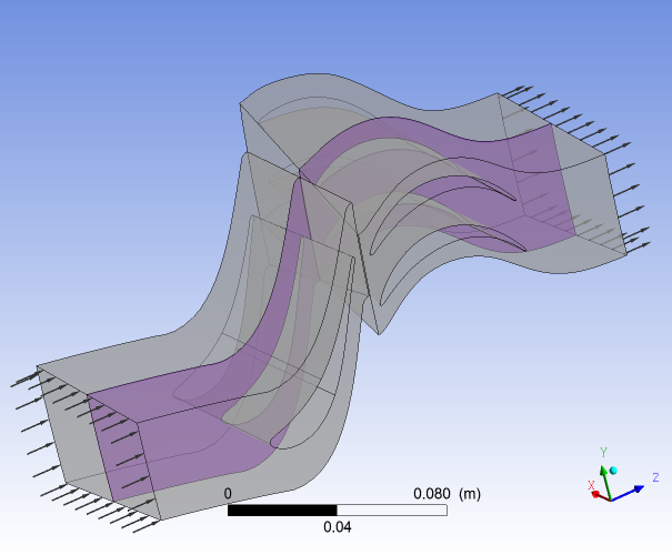
The goal of this tutorial is to set up a transient calculation of an axial turbine stage.
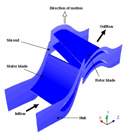
The stage contains 60 stator blades and 113 rotor blades. The following figure shows approximately half of the full geometry. The Inflow and Outflow labels show the location of the modeled section in Figure 14.1: Geometry subsection.
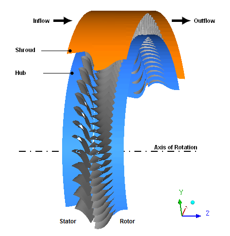
The geometry to be modeled consists of a single stator blade passage and two rotor blade passages. This is an approximation to the full geometry since the ratio of rotor blades to stator blades is close to, but not exactly, 2:1. In the stator blade passage a 6° section is being modeled (360°/60 blades), while in the rotor blade passage, a 6.372° section is being modeled (2*360°/113 blades). This produces a pitch ratio at the interface between the stator and rotor of 0.942. As the flow crosses the interface, it is scaled to enable this type of geometry to be modeled. This results in an approximation of the inflow to the rotor passage. Furthermore, the flow across the interface will not appear continuous due to the scaling applied.
You should always try to obtain a pitch ratio as close to 1 as possible in your model to minimize approximations, but this must be weighed against computational resources. A full machine analysis can be performed (modeling all rotor and stator blades), which always eliminates any pitch change, but will require significant computational time. For this geometry, a 1/4 machine section (28 rotor blades, 15 stator blades) would produce a pitch change of 1.009, but this would require a model about 15 times larger than in this tutorial example.
In this example, the rotor rotates about the Z axis at 523.6 rad/s while the stator and shroud are stationary. The tip gap between the rotor blades and the shroud is not included in the mesh. Periodic boundaries are used to enable only a small section of the full geometry to be modeled.
The important parameters of this problem are:
Total pressure = 0.265 bar
Static Pressure = 0.0662 bar
Total temperature = 328.5 K
The overall approach of this tutorial is to run a transient simulation using the Transient Rotor-Stator interface model initialized with the results of a steady-state simulation that uses the Frozen Rotor interface model. First, you will define a steady-state Frozen Rotor simulation using the Turbomachinery Wizard. The results of this simulation will be viewed using the Turbo Post feature. Next, you will rerun the steady-state Frozen Rotor simulation using an Exit Corrected Mass Flow Rate boundary condition. You will modify a copy of this steady-state Frozen Rotor simulation to define the transient simulation with the Transient Rotor-Stator interface model. After running the Transient Rotor-Stator simulation, you will create an animation showing domain movement.
If this is the first tutorial you are working with, it is important to review the following topics before beginning:
Create a working directory.
Ansys CFX uses a working directory as the default location for loading and saving files for a particular session or project.
Download the
axial.zipfile here .Unzip
axial.zipto your working directory.Ensure that the following tutorial input files are in your working directory:
rotor.grdstator.gtm
Set the working directory and start CFX-Pre.
For details, see Setting the Working Directory and Starting Ansys CFX in Stand-alone Mode.
You will first create the Frozen Rotor simulation.
The Turbomachinery wizard is designed to simplify the setup of turbomachinery simulations.
In CFX-Pre, select File > New Case.
Select Turbomachinery and click .
Select File > Save Case As.
Under File name, type
AxialIni.Click .
In the Basic Settings panel, configure the following setting(s):
Setting
Value
Machine Type
Axial Turbine
Analysis Type
> Type
Steady State
Click Next.
Two new components are required. As they are created, meshes are imported.
Right-click in the blank area and select Add Component from the shortcut menu.
Create a new component of type
Stationary, namedS1.Configure the following setting(s):
Setting
Value
Mesh
> File
stator.gtm [ a ]
Create a new component of type
Rotating, namedR1.Configure the following setting(s):
Setting
Value
Component Type
> Value
523.6 [radian s^-1]
Mesh
> File
rotor.grd [ a ]
Note: The components must be ordered as above (stator then rotor) in order for the interface to be created correctly. The order of the two components can be changed by right-clicking on
S1and selecting Move Component Up.When a component is defined, Turbo Mode will automatically select a list of regions that correspond to certain boundary types. This information should be reviewed in the Region Information section to ensure that all is correct. This information will be used to help set up boundary conditions and interfaces. The upper case turbo regions that are selected (for example,
HUB) correspond to the region names in the CFX-TASCflow grd file. CFX-TASCflow turbomachinery meshes use these names consistently.Click Passages and Alignment > Edit.
Configure the following setting(s):
Setting
Value
Passage and Alignment
> Passages/Mesh
> Passages per Mesh
2
Passage and Alignment
> Passages to Model
2
Passage and Alignment
> Passages in 360
113
Click Passages and Alignment > Done.
Configure the following setting(s):
Click Next.
In this section, you will set properties of the fluid domain and some solver parameters.
In the Physics Definition panel, configure the following setting(s):
Setting
Value
Fluid
Air Ideal Gas
Model Data
> Reference Pressure
0.25 [atm]
Model Data
> Heat Transfer
Total Energy
Model Data
> Turbulence
k-Epsilon
Inflow/Outflow Boundary Templates
> P-Total Inlet Mass Flow Outlet
(Selected)
Inflow/Outflow Boundary Templates
> Inflow
> P-Total
0 [atm]
Inflow/Outflow Boundary Templates
> Inflow
> T-Total
340 [K]
Inflow/Outflow Boundary Templates
> Inflow
> Flow Direction
Normal to Boundary
Inflow/Outflow Boundary Templates
> Outflow
> Mass Flow
Per Component
Inflow/Outflow Boundary Templates
> Outflow
> Mass Flow Rate
0.06 [kg s^-1]
Interface
> Default Type
Frozen Rotor
Solver Parameters
(Selected)
Solver Parameters
> Advection Scheme
High Resolution
Solver Parameters
> Convergence Control
Physical Timescale
Solver Parameters
> Physical Timescale
0.002 [s] [ a ]
Click Next.

CFX-Pre will try to create appropriate interfaces using the region names presented previously in the Region Information section. In this case, you should see that a periodic interface has been generated for both the rotor and the stator. These are required when modeling a small section of the true geometry. An interface is also required to connect the two components together across the frame change.
Review the various interfaces but do not change them.
Click Next.
CFX-Pre will try to create appropriate boundary conditions using the region names presented previously in the Region Information section. In this case, you should see a list of boundary conditions that have been generated. They can be edited or deleted in the same way as the interface connections that were set up earlier.
Review the various boundary definitions but do not change them.
Click Next.
Click Define Run
 .
.Configure the following setting(s):
Setting
Value
File name
AxialIni.def [ a ]
Click .
CFX-Solver Manager automatically starts and, on the Define Run dialog box, Solver Input File is set.
If using stand-alone mode, quit CFX-Pre, saving the simulation (
.cfx) file at your discretion.
Compared to previous tutorials, the mesh for this tutorial contains many more nodes (although it is still too coarse to perform a high quality CFD simulation). This results in a corresponding increase in solution time for the problem. Solving this problem in parallel is recommended, if possible.
More detailed information about setting up CFX to run in parallel is available in Flow Around a Blunt Body.
You can solve this example using Serial, Local Parallel or Distributed Parallel.
If you do not have a license to run CFX in parallel you can run in serial by clicking the Start Run button when CFX-Solver Manager has opened up. Solution time in serial is approximately 45 minutes on a 1 GHz processor.
Click Start Run on the Define Run dialog box.
CFX-Solver runs and attempts to obtain a solution. At the end of the run, a dialog box is displayed stating that the simulation has ended.
Select Post-Process Results.
If using stand-alone mode, select Shut down CFX-Solver Manager.
Click .
When you are finished, proceed to Viewing the Results Using CFD-Post.
To run in local parallel mode:
Set Run Mode to a parallel mode suitable for your environment; for example,
Intel MPI Local Parallel.If required, click Add Process
 to increase the maximum number of processes.
Ideally, the number of processes should not exceed the number of available processor cores. The number of processes used will be the number of partitions for the mesh.
Click Start Run.
Select the check box next to Post-Process Results when the completion message appears at the end of the run.
If using stand-alone mode, select the check box next to Shut down CFX-Solver Manager.
Click .
When you are finished, proceed to Viewing the Results Using CFD-Post.
Set Run Mode to a parallel mode suitable for your environment; for example,
Intel MPI Distributed Parallel.One partition should already be assigned to the host that you are logged into.
Click Insert Host
 to specify a new parallel host.
In Select Parallel Hosts, select another host name (this should be a machine that you can log into using the same user name).
Click Add, and then Close.
The names of the two selected machines should be listed in the Host Name column of the Define Run dialog box.
Click Start Run.
Select the check box next to Post-Process Results when the completion message appears at the end of the run.
If using stand-alone mode, select the check box next to Shut down CFX-Solver Manager.
Click .
When CFD-Post starts, the Domain Selector dialog box might appear. If it does, ensure that both the R1 and S1 domains are selected, then click to load the results from these domains.
The Turbo Post feature will be demonstrated in the following sections. This feature is designed to greatly reduce the effort taken to post-process turbomachinery simulations.
When initializing turbo components, span, a (axial), r (radial), and Theta coordinates are generated for each component. Therefore, after entering the Turbo workspace and initializing the turbo components, you will be ready to start using the turbo-specific features offered in the Turbo workspace immediately. These features include Turbo Tree View, Turbo Surface, Turbo Line and Turbo Plots.
To initialize Turbo Post, the properties of each component must be set up. This includes information about the inlet, outlet, hub, shroud, blade, and periodic regions. It also includes information about the number of instances of each turbo component needed to represent the full geometry around the rotation axis, and the number of blade passages in the mesh for each turbo component.
Click the Turbo tab.
The Turbo Initialization dialog box is displayed, and asks you whether you want to auto-initialize all components.
Note: If you do not see the Turbo Initialization dialog box, or as an alternative to using that dialog box, you can initialize all components by clicking the Initialize All Components button, which is visible initially by default, or after double-clicking the Initialization object in the Turbo tree view.
Click Yes.
In this case, the initialization works without problems. If there was a problem initializing a component, this would likely be indicated in the tree view.
Next, you will create a surface group colored by Pressure,
covering the blade and hub surfaces on three graphical instances of each domain.
From the main menu, select Insert > Location > Surface Group.
Click to accept the default name.
Configure the following setting(s):
Tab
Setting
Value
Geometry
Locations
R1 Blade, R1 Hub, S1 Blade, S1 Hub
Color
Mode
Variable
Variable
Pressure
Click Apply.
Click the Turbo tab.
Open Plots > 3D View for editing.
Configure the following setting(s):
Tab
Setting
Value
3D View
Graphical Instancing
> Domain
R1
Graphical Instancing
> # of Copies
3
Click Apply.
Configure the following setting(s):
Tab
Setting
Value
3D View
Graphical Instancing
> Domain
S1
Graphical Instancing
> # of Copies
3
Click Apply.
Click the Outline tab to see the surface group.
Note: The number of graphical instances can also be changed from the Outline tab, in the domain settings.
In this section, you will create a plot of pressure around the stator blade at a given spanwise location.
Click the Turbo tab.
In the Turbo tree view, double-click
Blade Loading.Click Apply.
This profile of the pressure curve is typical for turbomachinery applications.
When you are finished viewing the chart, return to the Outline tab and keep CFD-Post open.
You will now use a different outlet boundary condition, namely
the Exit Corrected Mass Flow Rate specification
for the R1 Outlet boundary, that will enable
you to specify the mass flow at the outlet at corrected conditions.
The Reference Pressure and Reference Temperature will be set to International
Standard Atmosphere (ISA) conditions (1 atm and 288.15 K).
The exit corrected mass flow is defined as:
 | (14–1) |
where,  and
and  are mass averaged values of total pressure and temperature
in the stationary frame at the outlet.
are mass averaged values of total pressure and temperature
in the stationary frame at the outlet.
The intent of this section is to obtain the same operating point with the exit corrected mass flow boundary condition as with the previous setup that used the mass flow boundary condition at the outlet. To do this you need to calculate, from the previous case’s results, the mass averaged values of total pressure and temperature at the outlet, in the stationary frame. These values along with the mass flow (0.06 kg s^-1) and the reference values mentioned above are substituted into Equation 14–1. The resulting value for the exit corrected mass flow is 0.3745 kg s^-1. You may want to verify this by doing the calculation yourself.
Ensure that the following tutorial input file is in your working directory:
AxialIni_001.res
Set the working directory and start CFX-Pre if it is not already open.
For details, see Setting the Working Directory and Starting Ansys CFX in Stand-alone Mode.
Open the results file named
AxialIni_001.res.Save the case as
AxialIni_Cor.cfxin your working directory.In the tree view, open
R1 Outletfor editing.Configure the following setting(s):
Tab
Setting
Value
Boundary Details
Mass And Momentum
> Option
Exit Corrected Mass Flow Rate
Mass And Momentum
> Mass Flow Rate
0.3745 [kg s^-1]
Mass And Momentum
> Ref. Temperature
288.15 [K]
Mass And Momentum
> Reference Pressure
1 [atm] [ a ]
Click .
Follow one of the next two procedures as appropriate:
Procedure 1: If Simulation Control > Execution Control does not appear in the outline tree view:
Click Define Run
.Configure the following setting(s):
Setting
Value
File name
AxialIni_Cor.def
Click .
CFX-Solver Manager automatically starts and, on the Define Run dialog box, Solver Input File is set.
Procedure 2: If Simulation Control > Execution Control appears in the outline tree view:
Click Execution Control
 .
.Configure the following setting(s):
Tab
Setting
Value
Run Definition
Input File Settings
> Solver Input File
AxialIni_Cor.def
Click .
Click Define Run
.
CFX-Solver Manager automatically starts and, on the Define Run dialog box, Solver Input File is set.
If using stand-alone mode, quit CFX-Pre, saving the simulation (
.cfx) file at your discretion.
As in the previous setup of the steady-state simulation for this case, solving the problem in parallel is recommended, if possible.
Ensure that the Define Run dialog box is displayed.
Select Run Mode > Intel MPI Local Parallel and click Start Run.
In CFX-Solver Manager, select Workspace > New Monitor in the main menu and click to accept the default name.
Configure the following setting(s):
Tab
Setting
Value
Plot Lines
Flow
> Boundary
> R1 Outlet
> P-Mass Boundary Flow on R1 Outlet (R1)
(Selected)
Click .
When the dialog box is displayed stating that the simulation has ended, click .
Note: The resulting plot of the P-Mass Boundary Flow on R1 Outlet (R1) vs. Accumulated Time Step converges to –0.06 on the Y axis. The exit corrected mass flow rate entered (0.3745 kg s^-1) for this run yields the same physical mass flow as used in the previous steady-state setup; this is expected. The value is negative because the flow is leaving the domain.
If you would like to convince yourself that the results are identical, you can proceed to the following section and do a case comparison in CFD-Post. If you do not want to compare the cases, proceed to Simulating the Stage with the Transient Rotor-Stator Model.
In this section you will compare the domain passages of the two cases.
With
AxialIni_001.resalready loaded in CFD-Post, select File > Load Results.In the Load Results File dialog box, select Keep current cases loaded, then select the file AxialIni_Cor_001.res. Click . If the Domain Selector dialog box appears, ensure that both the R1 and S1 domains are selected, and then click .
You should see the two cases beside one another in the 3D Viewer. Click the synchronize active view icon
 .
.Right-click within the 3D view and select Predefined Camera > Isometric View (Y up) to orient the views. Click Fit View
 to scale the blades appropriately within the 3D Viewer.
Next, you will create a plot on three graphical instances of each domain, as you did for the previous case.
Select Insert > Location > Surface Group from the main menu.
Click to accept the default name.
Configure the following setting(s):
Tab
Setting
Value
Geometry
Locations
> AxialIni_Cor_001
R1 Blade, R1 Hub, S1 Blade, S1 Hub [ a ]
Color
Mode
Variable
Variable
Pressure
Click Apply.
Click the Turbo tab.
Open Plots > 3D View for editing.
Configure the following setting(s):
Tab
Setting
Value
3D View
Graphical Instancing
> Domain
R1 (AxialIni_Cor_001)
Graphical Instancing
> # of Copies
3
Click Apply.
Note: If the image from the results of
AxialIni_Cor_001is not displayed in the 3D Viewer, select it from the drop-down list at the top of the viewer.Configure the following setting(s):
Tab
Setting
Value
3D View
Graphical Instancing
> Domain
S1 (AxialIni_Cor_001)
Graphical Instancing
> # of Copies
3
Click Apply.
Click the Outline tab to see the surface group.
To see both images, click the viewport icon and select
 . You may need to turn on the visibility of
 Surface Group 1in the tree view to compare the two surfaces.

After you have finished your comparison, close CFD-Post.
You will now create the Transient Rotor-Stator simulation. The existing steady-state Frozen Rotor simulation is modified to define the Transient Rotor-Stator simulation. If you have not already completed the Frozen Rotor simulation, refer to Simulating the Stage with the Steady-State Frozen Rotor Model before proceeding with the Transient Rotor-Stator simulation.
This section describes the step-by-step definition of the flow physics in CFX-Pre.
This step involves opening the original simulation and saving it to a different location.
Ensure that the following file is in your working directory:
AxialIni_001.res
Set the working directory and start CFX-Pre if it is not already running.
For details, see Setting the Working Directory and Starting Ansys CFX in Stand-alone Mode.
Open the results file named
AxialIni_001.res.Save the case as
Axial.cfxin your working directory.
You need to modify the domain to define a transient simulation. You are going to run for a time interval such that the rotor blades pass through 1 pitch (6.372°) using 10 time steps. This is generally too few time steps to obtain high quality results, but is sufficient for tutorial purposes. The time step size is calculated as follows:

Since 10 time steps are used over this interval each time step should be 2.124e-5 s.
Select Tools > Turbo Mode.
Basic Settings is displayed.
Configure the following setting(s):
Setting
Value
Analysis Type
> Type
Transient
Analysis Type
> Total Time
2.124e-4 [s]
Analysis Type
> Time Steps
2.124e-5 [s] [ a ]
Click Next.
Component Definition is displayed.
Click Next.
Physics Definition is displayed.
Configure the following setting(s):
Setting
Value
Fluid
Air Ideal Gas
Interface
> Default Type
Transient Rotor Stator
Note: A Transient Rotor-Stator calculation often runs long enough for the blades to pass through more than one pitch. In these cases, it may be useful to look at variable data averaged over the time interval required to complete 1 pitch. You can then compare data for each pitch rotation to see if a "steady state" has been achieved, or if the flow is still developing.
Click Next.
A warning message is displayed.
Click Yes.
Interface Definition is displayed.
Click Next.
Boundary Definition is displayed.
Click Next.
Final Operations is displayed.
Ensure that Operation is set to
Enter General Mode.Click Finish.
Initial values are required, but will be supplied later using a results file.
Click Output Control
 .
.Click the Trn Results tab.
In the Transient Results tree view, click Add new item
, set Name to Transient Results 1, and click OK.Configure the following setting(s):
Setting
Value
Option
Selected Variables
Output Variables List
Pressure, Velocity, Velocity in Stn Frame [ a ]
Output Frequency
> Option
Time Interval
Output Frequency
> Time Interval
2.124e-5 [s]
Click .
Click Execution Control
.Configure the following setting(s):
Tab
Setting
Value
Run Definition
Input File Settings
> Solver Input File
Axial.def [ a ]
Confirm that the rest of the execution control settings are set appropriately.
Click .
Click Define Run
.A warning will appear, due to a lack of initial values.
Initial values are required, but will be supplied later using a results file.
Click Yes.
If using stand-alone mode, quit CFX-Pre, saving the simulation (
.cfx) file at your discretion.
When the CFX-Solver Manager has started you will need to specify an initial values file before starting the CFX-Solver.
If you do not have a license, or do not want to run CFX in parallel, you can run it in serial. Solution time in serial is similar to the first part of this tutorial.
Under the Initial Values tab, select Initial Values Specification.
Under Initial Values Specification > Initial Values, select
Initial Values 1.Under Initial Values Specification > Initial Values > Initial Values 1 Settings > File Name, click Browse
 .
.Select
AxialIni_001.resfrom your working directory.Click Open.
Under Initial Values Specification > Use Mesh From, select
Solver Input File.Click Start Run.
CFX-Solver runs and attempts to obtain a solution. At the end of the run, a dialog box is displayed stating that the simulation has ended.
Select Post-Process Results.
If using stand-alone mode, select Shut down CFX-Solver Manager.
Click , then continue this tutorial from Monitoring the Run.
Follow the first 6 steps of the serial procedure above (in Serial Solution), then perform the local parallel or distributed parallel procedure from the first part of this tutorial (in Obtaining the Solution Using CFX-Solver Manager).
During the solution, look for the additional information that is provided for Transient Rotor-Stator runs. Each time the rotor is rotated to its next position, the number of degrees of rotation and the fraction of a pitch moved is given. You should see that after 10 time steps the rotor has been moved through 1 pitch.
To examine the transient interaction between the rotor and stator, you are going to create a blade-to-blade animation of pressure. A turbo surface will be used as the basis for this plot.
All the preprocessing will be done during the initialization of the turbo components. Only a few steps will therefore be required to display a surface of constant span and to create a turbo surface later on in this tutorial.
Click the Turbo tab.
The Turbo Initialization dialog box is displayed and asks you whether you want to auto-initialize all components.
Note: If you do not see the Turbo Initialization dialog box, or as an alternative to using that dialog box, you can initialize all components by clicking the Initialize All Components button, which is visible initially by default, or after double-clicking the Initialization object in the Turbo tree view.
Click Yes.
Both components (domains) are initialized based on the automatically selected turbo regions. When the process is complete, a green turbine icon appears next to each component entry in the list. Also, the viewer displays a green background mesh for each initialized component, visible when a component is selected.
Double-click
Component 1 (S1)and review the automatically-selected turbo regions and other data in the details view.Double-click
Component 2 (R1)and review the automatically-selected turbo regions and other data in the details view (including the Passages per Component setting on the Instancing tab, which should have a value of2).
In the Turbo tree view, double-click
Blade-to-Blade.Click Apply.
A surface of constant span appears, colored by pressure.
In the Turbo tree view, double-click Initialization.
Click Three Views.
Left view is 3D View, top right is Blade-to-Blade and bottom right is Meridional view.
Click Single View.
Select Insert > Location > Turbo Surface, and accept the default name.
Set Method to
Constant Spanand Value to0.5.Under the Color tab, set Mode to
Variable, Variable toPressure, Range toUser Specified, Min to-10000 [Pa], and Max to-7000 [Pa].Click Apply.
Next, you will use graphical instancing to view a larger section of the model.
In the Turbo tree view, double-click the 3D View object.
In the Graphical Instancing section of the form, set # of Copies to
6for R1.Click Apply.
In the Graphical Instancing section of the form, set # of Copies to
6for S1.Click Apply.
Return to the Outline tab and ensure that the turbo surface is visible again.
Start by loading the first time step:
Click Timestep Selector
 .
.Select time value 0.
Click Apply to load the time step. The rotor blades move to their starting positions. These positions are exactly 1 pitch from the blade positions that were previously displayed, so the blades will appear to be in the same positions.
Turn off the visibility of
Wireframe.Position the geometry as shown below, ready for the animation. During the animation the rotor blades will move to the right. Make sure you have at least two rotor blades out of view to the left side of the viewer. They will come into view during the animation.
Click Animation
 .
.The Animation dialog box appears.
Set Type to Keyframe Animation.
Click New
to create KeyFrameNo1.Select
KeyframeNo1, then set # of Frames to9, then press Enter while in the # of Frames box.Tip: Be sure to press Enter and confirm that the new number appears in the list before continuing.
Use the Timestep Selector to load the final time step.
In the Animation dialog box, click New
to create KeyframeNo2.Click More Animation Options
 to expand the Animation dialog
box.
to expand the Animation dialog
box.Click Options and set Transient Case to
TimeValue Interpolation. Click .The animation now contains a total of 11 frames (9 intermediate frames plus the two Keyframes), one for each of the available time values.
In the expanded Animation dialog box, select Save Movie.
Set Format to
MPEG1.Click Browse
,
next to the Save Movie box and then set the file
name to an appropriate file name.If frame 1 is not loaded (shown in the F: text box at the bottom of the Animation dialog box), click To Beginning
 to load it.
Wait for CFD-Post to finish loading the objects for this frame before proceeding.
Click Play the animation
 .
.It takes a while for the animation to be completed.
To view the movie file, you will need to use a media player that supports the MPEG format.
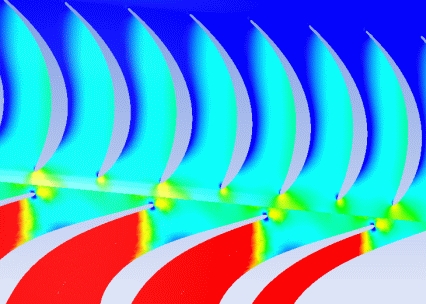
You will be able to see from the animation, and from the plots created previously, that the flow is not continuous across the interface. This is because a pitch change occurs. The relatively coarse mesh and the small number of time steps used in the transient simulation also contribute to this. The movie was created with a narrow pressure range compared to the global range, which exaggerates the differences across the interface.
You can produce a report for the turbine as follows:
Click File > Report > Report Templates.
In the Report Templates dialog box, select Turbine Report, then click Load.
The report will be generated automatically.
Click the Report Viewer tab (located below the viewer window).
A report appears.
Note that a valid report depends on valid turbo initialization.
In this section, you will export a surface from CFD-Post and then use this surface to create a Monitor Surface in CFX-Pre. This will enable you to see the solution update in CFD-Post as the solver progresses.
Load the
AxialIni_001.resfile created earlier.Click the Turbo tab.
A dialog box will ask if you want to auto-initialize all turbo components. Click Yes.
Select Insert > Location > Turbo Surface.
Set the Name to
R1 MidSpanand click OK.Under the Geometry tab, set Domains to
R1.Ensure that Method is set to
Constant Spanand Value is set to0.5to create a surface at the mid-span of the rotor.Click Apply.
A surface of constant span appears in the rotor.
Select Insert > Location > Turbo Surface.
Set the Name to
S1 MidSpanand click OK.Under the Geometry tab, set Domains to
S1.Ensure that Method is set to
Constant Spanand Value is set to0.5to create a surface at the mid-span of the rotor.Click Apply.
A surface of constant span appears in the stator. You now have two surfaces appearing in the viewer.
Click File > Export > Export.
The Export dialog box appears.
Set File to R1 MidSpan.csv.
Set Type to
Geometry Only.Set Locations to
R1 MidSpan.Click Save.
Repeat steps 1-5 for the stator surface naming the file S1 MidSpan.csv.
The surfaces have now been exported to your working directory and you can now close CFD-Post.
This section describes importing the surface into CFX-Pre and using it to define a rotating Monitor Surface.
Ensure that the following file is in your working directory:
Axial.cfx
Set the working directory and start CFX-Pre if it is not already running.
For details, see Setting the Working Directory and Starting Ansys CFX in Stand-alone Mode.
Open the file named
Axial.cfx.Save the case as
AxialMonitoring.cfxin your working directory.
In this section, you will load the previously created surfaces into CFX-Pre.
Select Insert > User Locations > User Surface.
The Insert User Surface dialog box appears.
Set the Name to
R1 MidSpan.Click Browse
.Select
R1 MidSpan.csvfrom your working directory.Click Open.
Select Visibility so you can see the surface in the graphics viewer.
Click OK.
Repeat steps 1-7, naming the user surface "
S1 MidSpan" and selectingS1 MidSpan.csvfrom your working directory.You can now see the two surfaces you created in CFD-Post in the CFX-Pre viewer.
In this section, you will create a coordinate frame that rotates at the same speed as the rotor. This will be used later in the Monitor Surface definition.
Select Insert > Coordinate Frame and accept the default name.
Configure the following setting(s):
Setting
Value
Option
Axis points
Frame Motion
(selected)
Frame Motion
> Option
Rotating
Frame Motion
> Angular Velocity
523.6 [radian s^-1]
Click OK.
Click Output Control
.Click the Monitor tab.
In the Monitor Surfaces group box, click Add new item
, set Name to S1 MonitorSurface, and click OK.Configure the following setting(s):
Setting
Value
Output Variables List
Pressure, Velocity
Output Location List
S1 MidSpan
Output Frequency
> Option
Every Timestep
Click .
Now you will create a Monitor Surface for the rotor.
In the Monitor Surfaces group box, click Add new item
, set Name to R1 MonitorSurface, and click OK.Configure the following setting(s):
Setting
Value
Coordinate Frame
Coord 1
[ a ]Output Variables List
Pressure, Velocity
Output Location List
R1 MidSpan
Output Frequency
> Option
Every Timestep
Click .
A benefit of using Monitor Surfaces is that solution data can be written for only those surfaces. This enables you to significantly reduce the size of any solution files by disabling the CFX-Solver from writing any volume data.
Click Output Control
.Click the Results tab.
Set Option to
None.Click .
Right-click
Analysis Typein the Outline tree view and select Edit.Set Time Steps > Timesteps to
2.124e-6 [s].Reducing the timestep size by a factor of 10 will make the simulation run for 100 timesteps. This allows more time to view the Monitor Surface in CFD-Post.
Click .
Right-click
Execution Controlin the Outline tree view and select Edit.Set Input File Settings > Solver Input File to AxialMonitoring.def.
This ensures that you do not overwrite any previously created .def file.
Click .
Click Define Run
.A warning will appear, due to a lack of initial values.
Initial values are required, but will be supplied later using a results file.
Click Yes.
If using stand-alone mode, quit CFX-Pre, saving the simulation (
.cfx) file at your discretion.
When the CFX-Solver Manager has started you will need to specify an initial values file before starting the CFX-Solver.
Ensure that Solver Input File is set to
AxialMonitoring.def.Under the Initial Values tab, select Initial Values Specification.
Under Initial Values Specification > Initial Values, select
Initial Values 1.Under Initial Values Specification > Initial Values > Initial Values 1 Settings > File Name, click Browse
.Select
AxialIni_001.resfrom your working directory.Click Open.
Under Initial Values Specification > Use Mesh From, select
Solver Input File.Click Start Run.
CFX-Solver runs and attempts to obtain a solution.
After the run has started, select Tools > Monitor Run with CFD-Post.
CFD-Post opens and loads the solution data.
In this section, you will create results objects and then allow CFD-Post to update and see the solution progress in real time.
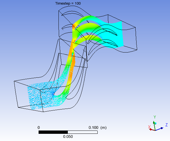
Select Insert > Text and accept the default name.
Select Embed Auto Annotation.
Set Type to
Timestep.Click Apply.
The current timestep will be displayed at the top of the viewer.
The Monitor Surface you defined in CFX-Pre has been pre-loaded into CFD-Post. You can
view it in the Outline tab under Other
Locations.
Select Other Locations > R1 MonitorSurface to
unhide it.
Double-click
R1 MonitorSurface.Under the Color tab set the Mode to
Variable.Set the Variable to
Pressure.Set the Range to
Local.Click Apply.
The contour is defined.
Select Monitor > Start Auto Update.
The contour now shows data and will regularly update to the data associated with the latest timestep generated by the solver. Notice how the rotor and Monitor Surface rotate together.
Object creation is prohibited in CFD-Post during Auto Update. You can look in CFX-Solver Manager to see if a timestep is almost complete.
Select Monitor > Stop Auto Update.
This stops the Auto Update and you can once again create and edit objects.
Select Insert > Vector and accept the default name.
Under the Geometry tab, set the Locations to
S1 MonitorSurface.Under the Color tab , set the Range to
Local.Click Apply.
The vector plot appears on the stator Monitor Surface. Now both results object are visible.
Wait until another timestep has completed and then select Monitor > Update Once.
This will load the most recently written solution data (most recent timestep in this case).
Select Monitor > Start Auto Update again.
You can watch the solution progress up until the run is finished.
In CFX-Solver Manager, you can stop the run by selecting Workspace > Stop Current Run at any time.