


This tutorial includes:
In this tutorial you will learn about:
Defining a non-Newtonian fluid.
Using the Moving Wall feature to apply a rotation to the fluid at a wall boundary.
|
Component |
Feature |
Details |
|---|---|---|
|
CFX-Pre |
User Mode |
General mode |
|
Analysis Type |
Steady State | |
|
Fluid Type |
General Fluid | |
|
Domain Type |
Single Domain | |
|
Turbulence Model |
Laminar | |
|
Heat Transfer |
None | |
|
Boundary Conditions |
Symmetry Plane | |
|
Wall: No-Slip | ||
|
Wall: Moving | ||
|
Timestep |
Auto Time Scale | |
|
CFD-Post |
Plots |
Sampling Plane |
|
Vector |
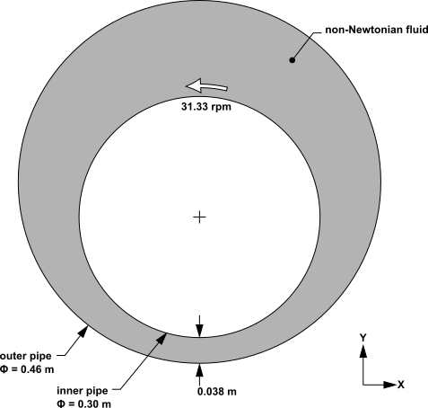
In this tutorial, a shear-thickening liquid rotates in a 2D eccentric annular pipe gap. The outer pipe remains stationary while the inner pipe rotates at a constant rate about its own axis, which is the Z axis. Both pipes have nonslip surfaces.
The fluid used in this simulation has material properties that are not a function of temperature. The ambient pressure is 1 atmosphere.
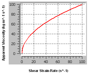
The shear-thickening liquid that is used in this tutorial obeys the Ostwald de Waele model with a viscosity consistency of 10.0 kg m-1 s-1, a Power Law index of 1.5, and a time constant of 1 s. This model is assumed to be valid for shear-strain rates ranging from 1.0E-3 s-1 to 100 s-1. The fluid has a density of 1.0E4 kg m-3. The viscosity is plotted over this range in Figure 13.2: Apparent Viscosity of a Shear-thickening Fluid.
A Newtonian fluid is a fluid for which shear stress is linearly proportional to shear-strain rate, with temperature held constant. For such a fluid, the dynamic viscosity is constant and equal to the shear stress divided by the shear-strain rate.
A non-Newtonian fluid is a fluid for which the shear stress in not linearly proportional to the shear-strain rate. For such fluids, the apparent viscosity is the ratio of shear stress to shear-strain rate for a given shear-strain rate.
A shear-thickening fluid is a type of non-Newtonian fluid for which the apparent viscosity increases with increasing shear-strain rate.
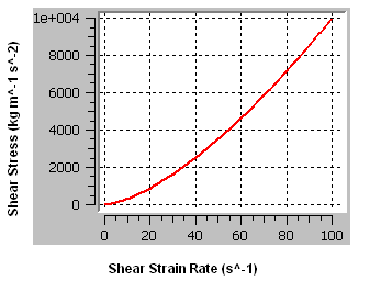
This tutorial involves a shear thickening fluid that obeys the Ostwald de Waele model between apparent viscosity and shear-strain rate:
 | (13–1) |
where  is the apparent viscosity,
  is the viscosity
consistency,
is the viscosity
consistency,  is the shear-strain rate,
  is
a normalizing time constant, and
is
a normalizing time constant, and  is the Power Law
index. Note that the units for
is the Power Law
index. Note that the units for  are not tied to the value of
  because
the quantity in parentheses is dimensionless.
because
the quantity in parentheses is dimensionless.
If this is the first tutorial you are working with, it is important to review the following topics before beginning:
Create a working directory.
Ansys CFX uses a working directory as the default location for loading and saving files for a particular session or project.
Download the
non_newton.zipfile here .Unzip
non_newton.zipto your working directory.Ensure that the following tutorial input file is in your working directory:
NonNewtonMesh.gtm
Set the working directory and start CFX-Pre.
For details, see Setting the Working Directory and Starting Ansys CFX in Stand-alone Mode.
In CFX-Pre, select File > New Case.
Select General and click .
Select File > Save Case As.
Under File name, type
NonNewton.Click .
Right-click
Meshand select Import Mesh > CFX Mesh.The Import Mesh dialog box appears.
Configure the following setting(s):
Setting
Value
File name
NonNewtonMesh.gtm
Click Open.
As stated in the problem description, the shear-thickening liquid
that is used in this tutorial obeys the Ostwald de Waele model with
a viscosity consistency ( ) of 10.0 kg m-1 s-1, a Power Law index (
 ) of 1.5,
and a time constant of 1 s. This model is assumed to be valid for
shear-strain rates ranging from 1.0E-3 s-1 to 100 s-1. The fluid has a density of
1.0E4 kg m-3.
) of 1.5,
and a time constant of 1 s. This model is assumed to be valid for
shear-strain rates ranging from 1.0E-3 s-1 to 100 s-1. The fluid has a density of
1.0E4 kg m-3.
Create a new material named
myfluid.Configure the following setting(s):
Tab
Setting
Value
Basic Settings
Thermodynamic State
(Selected)
Thermodynamic State
> Thermodynamic State
Liquid
Material Properties
Thermodynamic Properties
> Equation of State
> Molar Mass
1.0 [kg kmol^-1] [ a ]
Thermodynamic Properties
> Equation of State
> Density
1.0E+4 [kg m^-3]
Transport Properties
> Dynamic Viscosity
(Selected)
Transport Properties
> Dynamic Viscosity
> Option
Non Newtonian Model
Configure the following setting(s) under Transport Properties > Dynamic Viscosity > Non Newtonian Viscosity Model:
Setting
Value
Option
Ostwald de Waele
Viscosity Consistency
10.0 [kg m^-1 s^–1]
Min. Shear Strn. Rate
0.001 [s^-1]
Max. Shear Strn. Rate
100 [s^-1]
Time Constant
1 [s]
Power Law Index
1.5
Click .
The flow is expected to be laminar because the Reynolds number, based on the rotational speed, the maximum width of the pipe gap, and a representative viscosity (calculated using the shear-strain rate in the widest part of the gap, assuming a linear velocity profile), is approximately 30, which is well within the laminar-flow range.
From the problem description, the ambient pressure is 1 atmosphere.
Create a fluid domain that uses the non-Newtonian fluid you created in the previous section, and specify laminar flow with a reference pressure of 1 atmosphere:
Click Domain
 and set the name to
 NonNewton.Configure the following setting(s) of
NonNewton:Tab
Setting
Value
Basic Settings
Location
B8
Fluid and Particle Definitions
Fluid 1
Fluid and Particle Definitions
> Fluid 1
> Material
myfluid
Fluid Models
Heat Transfer
> Option
None
Turbulence
> Option
None (Laminar)
Click .
The inner and outer pipes both have nonslip surfaces. A rotating-wall boundary is required for the inner pipe. For the outer pipe, which is stationary, the default boundary is suitable. By not explicitly creating a boundary for the outer pipe, the latter receives the default wall boundary.
This tutorial models 2D flow in a pipe gap, where the latter is infinite in the Z direction. The flow domain models a thin 3D slice (in fact, just one layer of mesh elements) that has two surfaces of constant-Z coordinate that each require a boundary. Symmetry boundary conditions are suitable in this case, since there is no pressure gradient or velocity gradient in the Z direction.
From the problem description, the inner pipe rotates at 31.33 rpm about the Z axis. Create a wall boundary for the inner pipe that indicates this rotation:
Create a new boundary named
rotwall.Configure the following setting(s):
Tab
Setting
Value
Basic Settings
Boundary Type
Wall
Location
rotwall
Boundary Details
Mass And Momentum
> Option
No Slip Wall
Mass And Momentum
> Wall Velocity
(Selected)
Mass And Momentum
> Wall Velocity
> Option
Rotating Wall
Mass And Momentum
> Wall Velocity
> Angular Velocity
31.33 [rev min^-1]
Mass And Momentum
> Axis Definition
> Option
Coordinate Axis
Mass And Momentum
> Axis Definition
> Rotation Axis
Global Z
Click .
In order to simulate the presence of an infinite number of identical 2D slices while ensuring that the flow remains 2D, apply a symmetry boundary on the high-Z and low-Z sides of the domain:
Create a new boundary named
SymP1.Configure the following setting(s):
Tab
Setting
Value
Basic Settings
Boundary Type
Symmetry
Location
SymP1
Click .
Create a new boundary named
SymP2.Configure the following setting(s):
Tab
Setting
Value
Basic Settings
Boundary Type
Symmetry
Location
SymP2
Click .
The outer annulus surfaces will default to the no-slip stationary wall boundary.
A reasonable guess for the initial velocity field is a value of zero throughout the domain. In this case, the problem converges adequately and quickly with such an initial guess. If this were not the case, you could, in principle, create and use CEL expressions to specify a better approximation of the steady-state flow field based on the information given in the problem description.
Set a static initial velocity field:
Click Global Initialization
 .
.Configure the following setting(s):
Tab
Setting
Value
Global Settings
Initial Conditions
> Cartesian Velocity Components
> Option
Automatic with Value
Initial Conditions
> Cartesian Velocity Components
> U
0 [m s^-1]
Initial Conditions
> Cartesian Velocity Components
> V
0 [m s^-1]
Initial Conditions
> Cartesian Velocity Components
> W
0 [m s^-1]
Click .
Because this flow is low-speed, laminar, and because of the nature of the geometry, the solution converges very well. For this reason, set the solver control settings for a high degree of accuracy and a high degree of convergence.
Click Solver Control
 .
.Configure the following setting(s):
Click .
Click Define Run
 .
.Configure the following setting(s):
Setting
Value
File name
NonNewton.def
Click .
CFX-Solver Manager automatically starts and, on the Define Run dialog box, Solver Input File is set.
If using stand-alone mode, quit CFX-Pre, saving the simulation (
.cfx) file at your discretion.
When CFX-Pre has shut down and CFX-Solver Manager has started, you can obtain a solution to the CFD problem by following the instructions below:
Ensure that the Define Run dialog box is displayed.
Click Start Run.
CFX-Solver runs and attempts to obtain a solution. At the end of the run, a dialog box is displayed stating that the simulation has ended.
Select Post-Process Results.
If using stand-alone mode, select Shut down CFX-Solver Manager.
Click .
The following steps instruct you on how to create a vector plot showing the velocity values in the domain.
Right-click a blank area in the viewer and select Predefined Camera > View From -Z from the shortcut menu.
Create a new plane named
Plane 1.This plane will be used as a locator for a vector plot. To produce regularly-spaced sample points, create a circular sample plane, centered on the inner pipe, with a radius sufficient to cover the entire domain, and specify a reasonable number of sample points in the radial and theta directions. Note that the sample points are generated over the entire plane, and only those that are in the domain are usable in a vector plot.
Configure the following setting(s):
Tab
Setting
Value
Geometry
Definition
> Method
Point and Normal
Definition
> Point
0, 0, 0.015 [ a ]
Definition
> Normal
0, 0, 1
Plane Bounds
> Type
Circular
Plane Bounds
> Radius
0.3 [m]
Plane Type
Sample
Plane Type
> R Samples
32
Plane Type
> Theta Samples
24
Render
Show Faces
(Cleared)
Show Mesh Lines
(Selected)
Show Mesh Lines
> Color Mode
User Specified
Line Color
(Choose green, or some other color, to distinguish the sample plane from the
Wireframeobject.)Click Apply.
Examine the sample plane. The sample points are located at the line intersections. Note that many of the sample points are outside the domain. Only those points that are in the domain are usable for positioning vectors in a vector plot.
Turn off the visibility of
Plane 1.Create a new vector plot named
Vector 1onPlane 1.Configure the following setting(s):
Tab
Setting
Value
Geometry
Definition
> Locations
Plane 1
Definition
> Sampling
Vertex [ a ]
Definition
> Reduction
Reduction Factor
Definition
> Factor
1.0 [ b ]
Definition
> Variable
Velocity
Definition
> Boundary Data
Hybrid [ c ]
Symbol
Symbol Size
3 [ d ]
This causes the vectors to be located at the nodes of the sample plane you created previously. Note that the vectors can alternatively be spaced using other options that do not require a sample plane.
A reduction factor of 1.0 causes no reduction in the number of vectors so that there will be one vector per sample point.
The hybrid values are modified at the boundaries for postprocessing purposes.
Because CFD-Post normalizes the size of the vectors based on the largest vector, and because of the large variation of velocity in this case, the smallest velocity vectors would normally be too small to see clearly.
Click Apply.
In CFX-Pre, you created a shear-thickening liquid that obeys
the Ostwald de Waele model for shear-strain rates ranging from 1.0E-3
s-1 to 100 s-1. The values of dynamic viscosity, which are a function of the shear-strain
rate, were calculated as part of the solution. You can post-process
the solution using these values, which are stored in the Dynamic Viscosity variable. For example, you can use this
variable to color graphics objects.
Color Plane 1 using the Dynamic
Viscosity variable:
Turn on the visibility of
Plane 1.Edit
Plane 1.Configure the following setting(s):
Tab
Setting
Value
Color
Mode
Variable
Variable
Dynamic
Viscosity
Render
Show Faces
(Selected)
Click Apply
Try plotting Shear Strain Rate on the same
plane. Note that the distribution is somewhat different than that
of Dynamic Viscosity, as a consequence of the
nonlinear relationship (see Figure 13.2: Apparent Viscosity of a Shear-thickening Fluid).
When you have finished, quit CFD-Post.