


This tutorial includes:
In this tutorial you will learn about:
Creating and using a multicomponent fluid in CFX-Pre.
Using CEL to model a reaction in CFX-Pre.
Using an algebraic Additional Variable to model a scalar distribution.
Using a subdomain as the basis for component sources.
|
Component |
Feature |
Details |
|---|---|---|
|
CFX-Pre |
User Mode |
General mode |
|
Analysis Type |
Steady State | |
|
Fluid Type |
Variable Composition Mixture | |
|
Domain Type |
Single Domain | |
|
Turbulence Model |
k-Epsilon | |
|
Heat Transfer |
Thermal Energy | |
|
Particle Tracking |
Component Source | |
|
Boundary Conditions |
Inlet (Subsonic) | |
|
Outlet (Subsonic) | ||
|
Symmetry Plane | ||
|
Wall: Adiabatic | ||
|
Additional Variables |
| |
|
CEL (CFX Expression Language) |
| |
|
Timestep |
Physical Time Scale | |
|
CFD-Post |
Plots |
Isosurface |
|
Slice Plane |
Reaction engineering is one of the core components in the chemical industry. Optimizing reactor design leads to higher yields, lower costs and, as a result, higher profit.
This example demonstrates the capability of Ansys CFX to model basic reacting flows using a multicomponent fluid and CEL expressions.
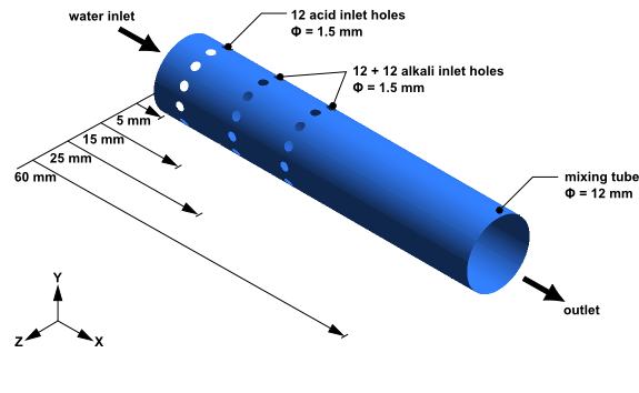
The geometry consists of a mixing tube with three rings with twelve holes in each ring.
The main inlet has water entering at 2 m/s with a temperature of 300 K. The pressure at the outlet is 1 atm.
Through the ring of holes nearest the inlet, a solution of dilute sulfuric acid enters at 2 m/s with a temperature of 300 K. Through each of the two other rings of holes, a solution of dilute sodium hydroxide enters at 2.923 m/s with a temperature of 300 K. The properties of the solution of sulfuric acid are shown in Table 15.1: Properties of the Dilute Sulfuric Acid Solution:
Table 15.1: Properties of the Dilute Sulfuric Acid Solution
|
Property |
Value |
|---|---|
|
Molar mass |
19.517 kg kmol^-1 |
|
Density |
1078 kg m^-3 |
|
Specific heat capacity |
4190 J kg^-1 K^-1 |
|
Dynamic Viscosity |
0.001 kg m^-1 s^-1 |
|
Thermal Conductivity |
0.6 W m^-1 K^-1 |
Through the remaining two rings of holes, a solution of dilute sodium hydroxide (an alkali) enters with a temperature of 300 K. The properties of the solution of sodium hydroxide are shown in Table 15.2: Properties of the Dilute Sodium Hydroxide Solution.
Table 15.2: Properties of the Dilute Sodium Hydroxide Solution
|
Property |
Value |
|---|---|
|
Molar mass |
18.292 kg kmol^-1 |
|
Density |
1029 kg m^-3 |
|
Specific heat capacity |
4190 J kg^-1 K^-1 |
|
Dynamic Viscosity |
0.001 kg m^-1 s^-1 |
|
Thermal Conductivity |
0.6 W m^-1 K^-1 |
The acid and alkali undergo an exothermic reaction to form a solution of sodium sulfate (a type of salt) and water according to the reaction:

Mixing the acid and alkali solutions in a stoichiometric ratio (and enabling them to react completely) would result in a salt water solution that would include water from each of the original solutions plus water produced during the reaction. The properties of this salt water product are shown in Table 15.3: Properties of the Salt Water Product.
Table 15.3: Properties of the Salt Water Product
|
Property |
Value |
|---|---|
|
Molar mass |
18.600 kg kmol^-1 |
|
Density |
1031 kg m^-3 |
|
Specific heat capacity |
4190 J kg^-1 K^-1 |
|
Dynamic Viscosity |
0.001 kg m^-1 s^-1 |
|
Thermal Conductivity |
0.6 W m^-1 K^-1 |
The heat of reaction is 460 kJ per kg of dilute acid solution.
The flow is assumed to be fully turbulent and turbulence is assumed to have a significant effect on the reaction rate.
After running the simulation, you will plot the distribution of pH in the tube, and determine the extent to which the pH is neutralized at the outlet. You will also plot mass fraction distributions of acid, alkali and product.
In order to reduce memory requirements and solution time, only a 30° slice of the geometry will be modeled, and symmetry boundary conditions will be applied to represent the remaining geometry.
The reaction between acid and alkali is represented as a single-step irreversible liquid-phase reaction:

Reagent  (dilute sulfuric acid) is injected
through a ring of holes near the start of the tube. As it flows along
the tube it reacts with Reagent
(dilute sulfuric acid) is injected
through a ring of holes near the start of the tube. As it flows along
the tube it reacts with Reagent  (dilute sodium hydroxide), which
is injected through a further two rings of holes downstream. The product,
(dilute sodium hydroxide), which
is injected through a further two rings of holes downstream. The product,  , remains
in solution.
, remains
in solution.
You will create a variable-composition mixture that contains water, the reactants, and the product. To model the reaction, you will use CEL expressions to govern the mass sources for the acid, alkali and product components. You will also use CEL expressions to govern the thermal energy source. Providing mass and energy sources over a volume requires a subdomain. Because the reaction may occur anywhere in the domain, you will create a subdomain that occupies the entire flow domain.
Note: You can also model this type of reaction using a reacting mixture as your fluid. For details, see Combustion and Radiation in a Can Combustor.
To model the pH, you will create an algebraic Additional Variable that is governed by a CEL expression for pH. The Additional Variable will be available in the solution results for analysis during postprocessing.
If this is the first tutorial you are working with, it is important to review the following topics before beginning:
Create a working directory.
Ansys CFX uses a working directory as the default location for loading and saving files for a particular session or project.
Download the
reactor.zipfile here .Unzip
reactor.zipto your working directory.Ensure that the following tutorial input files are in your working directory:
ReactorExpressions.cclReactorMesh.gtm
Set the working directory and start CFX-Pre.
For details, see Setting the Working Directory and Starting Ansys CFX in Stand-alone Mode.
In CFX-Pre, select File > New Case.
Select General and click .
Select File > Save Case As.
Under File name, type
Reactor.Click .
Right-click
Meshand select Import Mesh > CFX Mesh.The Import Mesh dialog box appears.
Configure the following setting(s):
Setting
Value
File name
ReactorMesh.gtm
Click Open.
In addition to providing template fluids, CFX allows you to create custom fluids for use in all your CFX models. A custom fluid may be defined as a pure substance, but may also be defined as a mixture, consisting of a number of transported fluid components. This type of fluid model is useful for applications involving mixtures, reactions, and combustion.
In order to define custom fluids, CFX-Pre provides the Material details view. This tool allows you to define your own fluids as pure substances, fixed composition mixtures or variable composition mixtures using a range of template property sets defined for common materials.
The mixing tube application requires a fluid made up from four separate materials (or components). The components are the reactants and products of a simple chemical reaction together with a neutral carrier liquid. You are first going to define the materials that take part in the reaction (acid, alkali and product) as pure substances. The neutral carrier liquid is water, and is already defined. Finally, you will create a variable composition mixture consisting of these four materials. This is the fluid that you will use in your simulation. A variable composition mixture (as opposed to a fixed composition mixture) is required because the proportion of each component will change throughout the simulation due to the reaction.
The properties of the dilute sulfuric acid solution were stated in the problem description.
Create a new material named
acid.Configure the following setting(s):
Tab
Setting
Value
Basic Settings
Option
Pure Substance
Thermodynamic State
(Selected)
Thermodynamic State
> Thermodynamic State
Liquid
Material Properties
Option
General Material
Thermodynamic Properties
> Equation of State
> Option
Value
Thermodynamic Properties
> Equation of State
> Molar Mass
19.517 [kg kmol^-1] [ a ]
Thermodynamic Properties
> Equation of State
> Density
1078 [kg m^-3]
Thermodynamic Properties
> Specific Heat Capacity
(Selected)
Thermodynamic Properties
> Specific Heat Capacity
> Option
Value
Thermodynamic Properties
> Specific Heat Capacity
> Specific Heat Capacity
4190 [J kg^-1 K^-1]
Transport Properties
> Dynamic Viscosity
(Selected)
Transport Properties
> Dynamic Viscosity
> Option
Value
Transport Properties
> Dynamic Viscosity
> Dynamic Viscosity
0.001 [kg m^-1 s^-1]
Transport Properties
> Thermal Conductivity
(Selected)
Transport Properties
> Thermal Conductivity
> Option
Value
Transport Properties
> Thermal Conductivity
> Thermal Conductivity
0.6 [W m^-1 K^-1]
Click .
The properties of the dilute sodium hydroxide solution were stated in the problem description.
Create a new material named
alkali.Configure the following setting(s):
Tab
Setting
Value
Basic Settings
Option
Pure Substance
Thermodynamic State
(Selected)
Thermodynamic State
> Thermodynamic State
Liquid
Material Properties
Option
General Material
Thermodynamic Properties
> Equation of State
> Option
Value
Thermodynamic Properties
> Equation of State
> Molar Mass
18.292 [kg kmol^-1]
Thermodynamic Properties
> Equation of State
> Density
1029 [kg m^-3]
Thermodynamic Properties
> Specific Heat Capacity
(Selected)
Thermodynamic Properties
> Specific Heat Capacity
> Option
Value
Thermodynamic Properties
> Specific Heat Capacity
> Specific Heat Capacity
4190 [J kg^-1 K^-1]
Transport Properties
> Dynamic Viscosity
(Selected)
Transport Properties
> Dynamic Viscosity
> Option
Value
Transport Properties
> Dynamic Viscosity
> Dynamic Viscosity
0.001 [kg m^-1 s^-1]
Transport Properties
> Thermal Conductivity
(Selected)
Transport Properties
> Thermal Conductivity
> Option
Value
Transport Properties
> Thermal Conductivity
> Thermal Conductivity
0.6 [W m^-1 K^-1]
Click .
The properties of the salt water product were stated in the problem description.
Create a new material named
product.Configure the following setting(s):
Tab
Setting
Value
Basic Settings
Option
Pure Substance
Thermodynamic State
(Selected)
Thermodynamic State
> Thermodynamic State
Liquid
Material Properties
Option
General Material
Thermodynamic Properties
> Equation of State
> Option
Value
Thermodynamic Properties
> Equation of State
> Molar Mass
18.600 [kg kmol^-1]
Thermodynamic Properties
> Equation of State
> Density
1031 [kg m^-3]
Thermodynamic Properties
> Specific Heat Capacity
(Selected)
Thermodynamic Properties
> Specific Heat Capacity
> Option
Value
Thermodynamic Properties
> Specific Heat Capacity
> Specific Heat Capacity
4190 [J kg^-1 K^-1]
Transport Properties
> Dynamic Viscosity
(Selected)
Transport Properties
> Dynamic Viscosity
> Option
Value
Transport Properties
> Dynamic Viscosity
> Dynamic Viscosity
0.001 [kg m^-1 s^-1]
Transport Properties
> Thermal Conductivity
(Selected)
Transport Properties
> Thermal Conductivity
> Option
Value
Transport Properties
> Thermal Conductivity
> Thermal Conductivity
0.6 [W m^-1 K^-1]
Click .
Define a variable composition mixture by combining water with
the three materials you have defined: acid, alkali, product.
Create a new material named
mixture.Configure the following setting(s):
Tab
Setting
Value
Basic Settings
Option
Variable Composition Mixture
Material Group
User, Water Data
Materials List
Water, acid, alkali, product
Thermodynamic State
(Selected)
Thermodynamic State
> Thermodynamic State
Liquid
Click .
You are going to use an Additional Variable to model the distribution of pH in the mixing tube. You can create Additional Variables and use them in selected fluids in your domain.
Create a new Additional Variable named
MixturePH.Configure the following setting(s):
Tab
Setting
Value
Basic Settings
Variable Type
Specific
Units
[ ]
Tensor Type
Scalar
Click .
This Additional Variable is now available for use when you create or modify a domain. You will set other properties of the Additional Variable, including how it is calculated, when you apply it to the domain later in this tutorial.
This section includes:
The first section shows a derivation for the mass-based stoichiometric ratio of alkali solution to acid solution. This ratio is used for calculating various quantities throughout this tutorial.
The second subsection (Reaction Source Terms) shows you how reactions and reaction kinetics can be formulated using the Eddy Break Up (EBU) model.
The third subsection (Calculating pH), shows you how pH is calculated.
In the fourth subsection (Loading the Expressions to Model the Reaction and pH) you will use a provided file to load CEL expressions for the reaction source terms and the pH.
The mass-based stoichiometric ratio of alkali solution to acid solution is a quantity that is used in several calculations in this tutorial. It represents the mass ratio of alkali solution to acid solution which leads to complete reaction with no excess alkali or acid (that is, neutral pH). This section of the tutorial shows you how to calculate the stoichiometric ratio, and introduces other quantities that are used in this tutorial.
The alkali solution contains water and sodium hydroxide. In the alkali solution, it is assumed that the sodium hydroxide molecules completely dissociate into ions according to the following reaction:

The acid solution contains water and sulfuric acid. In the acid solution, it is assumed that the sulfuric acid molecules completely dissociate into ions according to the following reaction:

The  ions and
  ions react
to form sodium sulfate (a type of salt) and water according to the
reaction:
ions react
to form sodium sulfate (a type of salt) and water according to the
reaction:

Note that this reaction requires the ions from two molecules of sodium hydroxide and the ions from one molecule of sulfuric acid. The stoichiometric ratio for the dry alkali and acid molecules is 2-to-1.
Instead of modeling dry molecules of alkali and acid, this tutorial
models solutions that contain these molecules (in dissociated form)
plus water. The calculations used to model the alkali-acid reactions,
and to measure the pH, require a mass-based stoichiometric ratio,  , that expresses
the mass ratio between the alkali solution and the acid solution required
for complete reaction of all of the (dissociated) alkali and acid
molecules within them.
, that expresses
the mass ratio between the alkali solution and the acid solution required
for complete reaction of all of the (dissociated) alkali and acid
molecules within them.
Using  to denote
  and
and  to denote
  , the ratio
  can be computed as the ratio of the following two
masses:
can be computed as the ratio of the following two
masses:
The mass of alkali solution required to contain 2 kmol of

The mass of acid solution required to contain 1 kmol of

A formula for calculating  is:
is:
 | (15–1) |
where:
 is the concentration of
  in kmol/kg solution (equal to the concentration
of
in kmol/kg solution (equal to the concentration
of  in kmol/kg solution).
 is the concentration of
  in kmol/kg solution
(equal to the concentration of
in kmol/kg solution
(equal to the concentration of  in kmol/kg solution).
The molar mass of the alkali solution (given as 18.292 kg/kmol solution) is a weighted average of the molar masses of water (18.015 kg/kmol) and dry sodium hydroxide (39.9971 kg/kmol), with the weighting in proportion to the number of each type of molecule in the solution. You can compute the fraction of the molecules in the solution that are sodium hydroxide as:

 can then
be calculated as follows:
can then
be calculated as follows:

The molar mass of the acid solution (given as 19.517 kg/kmol solution) is a weighted average of the molar masses of water (18.015 kg/kmol) and dry sulfuric acid (98.07848 kg/kmol), with the weighting in proportion to the number of each type of molecule in the solution. You can compute the fraction of the molecules in the solution that are sulfuric acid as:

 can then be calculated as follows:

Substituting the values for  and
and  into Equation 15–1 yields the
mass-based stoichiometric ratio of alkali solution to acid solution:
into Equation 15–1 yields the
mass-based stoichiometric ratio of alkali solution to acid solution:  .
.
The reaction and reaction rate are modeled using a basic Eddy Break Up formulation for the component and energy sources. For example, the transport equation for the mass fraction of acid solution is:
 | (15–2) |
where  is time,
  is velocity,
  is
the local density of the variable composition mixture,
is
the local density of the variable composition mixture,  is the mass fraction
of the acid solution in the mixture,
is the mass fraction
of the acid solution in the mixture,  is the kinematic diffusivity of the acid solution
through the mixture, and
is the kinematic diffusivity of the acid solution
through the mixture, and  is the stoichiometric ratio of
alkali solution to acid solution based on mass fraction. The right-hand
side represents the mass source term that is applied to the transport
equation for the acid solution. The left-hand side consists of the
transient, advection and diffusion terms.
is the stoichiometric ratio of
alkali solution to acid solution based on mass fraction. The right-hand
side represents the mass source term that is applied to the transport
equation for the acid solution. The left-hand side consists of the
transient, advection and diffusion terms.
In addition to specifying the sources for the acid solution and alkali solution, source coefficients will also be used in order to enhance solution convergence. For details, see the technical note at the end of this section.
The reaction rate is computed as:

where  is the turbulence kinetic energy,
and
is the turbulence kinetic energy,
and  is the turbulence eddy dissipation.
Note that the reaction rate appears on the right-hand side of Equation 15–2. The reaction rate is also
used to govern the rate of thermal energy production according to
the relation:
is the turbulence eddy dissipation.
Note that the reaction rate appears on the right-hand side of Equation 15–2. The reaction rate is also
used to govern the rate of thermal energy production according to
the relation:

From the problem description, the heat of reaction is 460 kJ per kg of acid solution.
Note: This is a technical note, for reference only.
A source is fully specified by an expression for its value  .
.
A source coefficient  is optional, but can be specified
to provide convergence enhancement or stability for strongly-varying
sources. The value of
is optional, but can be specified
to provide convergence enhancement or stability for strongly-varying
sources. The value of  may affect the rate of convergence
but should not affect the converged results.
may affect the rate of convergence
but should not affect the converged results.
If no suitable value is available for  , the solution time
scale or time step can still be reduced to help improve convergence
of difficult source terms.
, the solution time
scale or time step can still be reduced to help improve convergence
of difficult source terms.
Important:
 must never be positive.
An optimal value for  when solving an individual equation
for a positive variable
when solving an individual equation
for a positive variable  with a source
  whose strength
decreases with increasing
whose strength
decreases with increasing  is
is

Where this derivative cannot be computed easily,

may be sufficient to ensure convergence. (This is the form used for the acid solution and alkali solution mass source coefficients in this tutorial.)
Another useful formula for  is
is

where  is a local estimate for the source
time scale. Provided that the source time scale is not excessively
short compared to flow or mixing time scales, this may be a useful
approach for controlling sources with positive feedback (
is a local estimate for the source
time scale. Provided that the source time scale is not excessively
short compared to flow or mixing time scales, this may be a useful
approach for controlling sources with positive feedback ( ) or sources that do not depend
directly on the solved variable
) or sources that do not depend
directly on the solved variable  .
.
The pH (or acidity) of the mixture is a function of the volume-based
concentration of  ions. The latter can be computed using
the following two equations, which are based on charge conservation
and equilibrium conditions, respectively:
ions. The latter can be computed using
the following two equations, which are based on charge conservation
and equilibrium conditions, respectively:


(where  is the constant
for the self-ionization of water (1.0E-14 kmol2 m-6)).
is the constant
for the self-ionization of water (1.0E-14 kmol2 m-6)).
You can substitute one equation into the other to obtain the following quadratic equation:

which can be rearranged into standard quadratic form as:

The quadratic equation can be solved for  using
the equation
using
the equation  where
where  ,
,  and
and  .
.
The volume-based concentrations of  and
and  are required to calculate
  , and can be calculated from the mass fractions of
the components using the following expressions:
, and can be calculated from the mass fractions of
the components using the following expressions:


where:
 is the
concentration of
is the
concentration of  in kmol/m^3.
 is the concentration
of
is the concentration
of  in kmol/m^3.
 is the concentration of
  in kmol/kg solution
(equal to the concentration of
in kmol/kg solution
(equal to the concentration of  in kmol/kg solution).
 is the concentration of
  in kmol/kg solution (equal to the concentration
of
in kmol/kg solution (equal to the concentration
of  in kmol/kg solution).
 is the local density of the variable
composition mixture.
is the local density of the variable
composition mixture. is the mass-based stoichiometric
ratio of alkali solution to acid solution.
is the mass-based stoichiometric
ratio of alkali solution to acid solution.
Note that the second expression above can be re-written by substituting
for  using Equation 15–1. The result
is:
using Equation 15–1. The result
is:

After solving for the concentration of  ions, the pH can be
computed as:
ions, the pH can be
computed as:

In order to set a limit on pH for calculation purposes, the following relation will be used in this tutorial:

Load the expressions required to model the reaction sources and pH:
Select File > Import > CCL.
Ensure that Import Method is set to Append.
Select ReactorExpressions.ccl, which should be in your working directory.
Click Open.
Observe the expressions listed in the tree view of CFX-Pre. Some expressions are used to support other expressions. The main expressions are:
|
Expression Name |
Description |
Supporting Expressions |
|---|---|---|
|
pH |
The pH of the mixture. |
Hions, a, b, c, Yions, Xions, alpha, i |
|
HeatSource |
The thermal energy released from the reaction. |
HeatReaction, Rate |
|
AcidSource |
The rate of production of acid due to the reaction (always negative or zero). |
Rate |
|
AcidSourceCoeff |
The source coefficient for AcidSource (to enhance convergence). |
AcidSource |
|
AlkaliSource |
The rate of production of alkali due to the reaction (always negative or zero). |
Rate |
|
AlkaliSourceCoeff |
The source coefficient for AlkaliSource (to enhance convergence). |
AlkaliSource |
|
ProductSource |
The rate of production of salt water product (always positive or zero). |
Rate |
Note that the expressions do not refer to a particular fluid
since there is only a single fluid (which happens to be a multicomponent
fluid). In a multiphase simulation you must prefix variables with
a fluid name, for example Mixture.acid.mf instead of acid.mf.
In this section, you will create a fluid domain that contains the variable composition mixture and the Additional Variable that you created earlier. The Additional Variable will be set up as an algebraic equation with values calculated from the CEL expression for pH.
Edit
Case Options>Generalin the Outline tree view and ensure that Automatic Default Domain is turned on.A domain named
Default Domainshould now appear under theSimulationbranch.Edit
Default Domain.Under the Fluid and Particle Definitions setting, delete
Fluid 1and create a new fluid definition calledMixture.Configure the following setting(s):
Tab
Setting
Value
Basic Settings
Location and Type
> Location
B1.P3
Location and Type
> Domain Type
Fluid Domain
Fluid and Particle Definitions
Mixture
Fluid and Particle Definitions
> Mixture
> Material
mixture
Domain Models
> Pressure
> Reference Pressure
1 [atm]
Fluid Models
Heat Transfer
> Option
Thermal Energy
Turbulence
> Option
k-Epsilon
Component Models
> Component
acid
Component Models
> Component
> acid
> Option
Transport Equation
Component Models
> Component
> acid
> Kinematic Diffusivity
(Selected)
Component Models
> Component
> acid
> Kinematic Diffusivity
> Kinematic Diffusivity
0.001 [m^2 s^-1]
Use the same Option and Kinematic Diffusivity settings for
alkaliandproductas you have just set foracid.For
Water, set Option toConstraintas follows:Tab
Setting
Value
Fluid Models
Component Models
> Component
Water
Component Models
> Component
> Water
> Option
Constraint
One component must always use
Constraint. This is the component used to balance the mass fraction equation; the sum of the mass fractions of all components of a fluid must equal unity.Configure the following setting(s) to apply the Additional Variable that you created earlier:
Tab
Setting
Value
Fluid Models
Additional Variable Models
> Additional Variable
> MixturePH
(Selected)
Additional Variable Models
> Additional Variable
> MixturePH
> Option
Algebraic Equation [ a ]
Additional Variable Models
> Additional Variable
> MixturePH
> Add. Var. Value
pH
The other possible options either involve a transport equation to transport the Additional Variable in the flow field, or a Vector Algebraic Equation, which is for vector quantities. The Algebraic Equation is suitable because it allows the calculation of pH as a function of existing variables and expressions.
Click .
To provide the correct modeling for the chemical reaction you
need to define mass fraction sources for the fluid components acid, alkali, and product. To do this, you need to create a subdomain where the relevant sources
can be specified. In this case, sources need to be provided within
the entire domain of the mixing tube since the reaction occurs throughout
the domain.
Ensure that you have loaded the CEL expressions from the provided file.
The expressions should be listed in the tree view.
Create a new subdomain named
sources.Configure the following setting(s):
Tab
Setting
Value
Basic Settings
Location
B1.P3 [ a ]
Sources
Sources
(Selected)
Sources
> Equation Sources
acid.mf
Sources
> Equation Sources
> acid.mf
(Selected)
Sources
> Equation Sources
> acid.mf
> Option
Source
Sources
> Equation Sources
> acid.mf
> Source
AcidSource
Sources
> Equation Sources
> acid.mf
> Source Coefficient
(Selected)
Sources
> Equation Sources
> acid.mf
> Source Coefficient
> Source Coefficient
AcidSourceCoeff
Sources
> Equation Sources
alkali.mf
Sources
> Equation Sources
> alkali.mf
(Selected)
Sources
> Equation Sources
> alkali.mf
> Option
Source
Sources
> Equation Sources
> alkali.mf
> Source
AlkaliSource
Sources
> Equation Sources
> alkali.mf
> Source Coefficient
(Selected)
Sources
> Equation Sources
> alkali.mf
> Source Coefficient
> Source Coefficient
AlkaliSourceCoeff
Sources
> Equation Sources
Energy
Sources
> Equation Sources
> Energy
(Selected)
Sources
> Equation Sources
> Energy
> Option
Source
Sources
> Equation Sources
> Energy
> Source
HeatSource
Sources
> Equation Sources
product.mf
Sources
> Equation Sources
> product.mf
(Selected)
Sources
> Equation Sources
> product.mf
> Option
Source
Sources
> Equation Sources
> product.mf
> Source
ProductSource
Sources
> Equation Sources
> product.mf
> Source Coefficient
(Selected)
Sources
> Equation Sources
> product.mf
> Source Coefficient
> Source Coefficient
0 [kg m^-3 s^-1]
Click .
Add boundary conditions for all boundaries except the mixing tube wall; the latter will receive the default wall condition. Many of the required settings were given in the problem description. Since the fluid in the domain is a multicomponent fluid, you can control which component enters at each inlet by setting mass fractions appropriately. Note that water is the constraint material; its mass fraction is computed as unity minus the sum of the mass fractions of the other components.
Create a boundary for the water inlet using the given information:
Create a new boundary named
InWater.Configure the following setting(s):
Tab
Setting
Value
Basic Settings
Boundary Type
Inlet
Location
InWater
Boundary Details
Mass and Momentum
> Option
Normal Speed
Mass and Momentum
> Normal Speed
2 [m s^-1]
Heat Transfer
> Option
Static Temperature
Heat Transfer
> Static Temperature
300 [K]
Leave mass fractions for all components set to zero. Since
Wateris the constraint fluid, it will be automatically given a mass fraction of 1 on this inlet.Click .
Create a boundary for the acid solution inlet hole using the given information:
Create a new boundary named
InAcid.Configure the following setting(s):
Tab
Setting
Value
Basic Settings
Boundary Type
Inlet
Location
InAcid
Boundary Details
Mass and Momentum
> Option
Normal Speed
Mass and Momentum
> Normal Speed
2 [m s^-1]
Heat Transfer
> Option
Static Temperature
Heat Transfer
> Static Temperature
300 [K]
Component Details
acid
Component Details
> acid
> Mass Fraction
1.0
Component Details
alkali
Component Details
> alkali
> Mass Fraction
0
Component Details
product
Component Details
> product
> Mass Fraction
0
Click .
Create a boundary for the alkali solution inlet holes using the given information:
Create a new boundary named
InAlkali.Configure the following setting(s):
Tab
Setting
Value
Basic Settings
Boundary Type
Inlet
Location
InAlkali
Boundary Details
Mass and Momentum
> Option
Normal Speed
Mass and Momentum
> Normal Speed
2.923 [m s^-1]
Heat Transfer
> Option
Static Temperature
Heat Transfer
> Static Temperature
300 [K]
Component Details
> acid
(Selected)
Component Details
> acid
> Mass Fraction
0
Component Details
> alkali
(Selected)
Component Details
> alkali
> Mass Fraction
1
Component Details
> product
(Selected)
Component Details
> product
> Mass Fraction
0
Click .
Create a subsonic outlet at 1 atm (which is the reference pressure that was set in the domain definition):
Create a new boundary named
out.Configure the following setting(s):
Tab
Setting
Value
Basic Settings
Boundary Type
Outlet
Location
out
Boundary Details
Mass and Momentum
> Option
Static Pressure
Mass and Momentum
> Relative Pressure
0 [Pa]
Click .
The geometry models a 30° slice of the full geometry. Create two symmetry boundaries, one for each side of the geometry, so that the simulation models the entire geometry.
Create a new boundary named
sym1.Configure the following setting(s):
Tab
Setting
Value
Basic Settings
Boundary Type
Symmetry
Location
sym1
Click .
Create a new boundary named
sym2.Configure the following setting(s):
Tab
Setting
Value
Basic Settings
Boundary Type
Symmetry
Location
sym2
Click .
Note that, in this case, a periodic interface can be used as an alternative to the symmetry boundary conditions.
The values for acid, alkali, and product will be initialized to 0. Since Water is the constrained component, it will make up the
remaining mass fraction which, in this case, is 1.
Since the inlet velocity is 2 m/s, a reasonable guess for the initial velocity is 2 m/s.
Click Global Initialization
 .
.Configure the following setting(s):
Tab
Setting
Value
Global Settings
Initial Conditions
> Cartesian Velocity Components
> Option
Automatic with Value
Initial Conditions
> Cartesian Velocity Components
> U
2 [m s^-1]
Initial Conditions
> Cartesian Velocity Components
> V
0 [m s^-1]
Initial Conditions
> Cartesian Velocity Components
> W
0 [m s^-1]
Initial Conditions
> Component Details
acid
Initial Conditions
> Component Details
> acid
> Option
Automatic with Value
Initial Conditions
> Component Details
> acid
> Mass Fraction
0
Initial Conditions
> Component Details
alkali
Initial Conditions
> Component Details
> alkali
> Option
Automatic with Value
Initial Conditions
> Component Details
> alkali
> Mass Fraction
0
Initial Conditions
> Component Details
product
Initial Conditions
> Component Details
> product
> Option
Automatic with Value
Initial Conditions
> Component Details
> product
> Mass Fraction
0
Click .
Click Solver Control
 .
.Configure the following setting(s):
Tab
Setting
Value
Basic Settings
Advection Scheme
> Option
High Resolution
Convergence Control
> Max. Iterations
50
Convergence Control
> Fluid Timescale Control
> Timescale Control
Physical Timescale
Convergence Control
> Fluid Timescale Control
> Physical Timescale
0.01 [s] [ a ]
Click .
Click Define Run
 .
.Configure the following setting(s):
Setting
Value
File name
Reactor.def
Click .
CFX-Solver Manager automatically starts and, on the Define Run dialog box, Solver Input File is set.
If using stand-alone mode, quit CFX-Pre, saving the simulation (
.cfx) file at your discretion.
When CFX-Solver Manager has started, obtain a solution to the CFD problem as follows:
Ensure that the Define Run dialog box is displayed.
Select Double Precision.
This provides the precision required to evaluate the expression for pH.
Click Start Run.
CFX-Solver runs and attempts to obtain a solution. At the end of the run, a dialog box is displayed stating that the simulation has ended.
Select Post-Process Results.
If using stand-alone mode, select Shut down CFX-Solver Manager.
Click .
To see the nature and extent of the reaction process, examine the pH, the mass fractions, and turbulence quantities on a plane as follows:
Create an XY slice plane through Z = 0.
Turn off the visibility of the plane you just created.
Create contour plots of the following variables on that plane:
MixturePHacid.Mass Fractionalkali.Mass Fractionproduct.Mass FractionTurbulence Kinetic EnergyTurbulence Eddy Dissipation
Create an expression for
Turbulence Eddy Dissipation/Turbulence Kinetic Energy, then create a variable using the expression (only variables can be plotted) and create a contour plot using that variable. This quantity is an indicator of the reaction rate — it represents 1 / mixing timescale.