


This tutorial includes:
In this tutorial you will learn about:
Setting Up a Combustion Model in CFX-Pre.
Using a Reacting Mixture.
Using the Eddy Dissipation combustion model.
Using the P1 radiation model.
Creating thin surfaces for the inlet vanes.
Using chemistry postprocessing.
Changing object color maps in CFD-Post to prepare a grayscale image.
Using the function calculator in CFD-Post.
Creating a vector plot in CFD-Post.
Component | Feature | Details |
|---|---|---|
CFX-Pre | User Mode | General mode |
Analysis Type | Steady State | |
Fluid Type | Reacting Mixture | |
Domain Type | Single Domain | |
Turbulence Model | k-Epsilon | |
Heat Transfer | Thermal Energy | |
Combustion | ||
Radiation | ||
Boundary Conditions | Inlet (Subsonic) | |
Outlet (Subsonic) | ||
Wall: No-Slip | ||
Wall: Adiabatic | ||
Wall: Thin Surface | ||
Timestep | Physical Time Scale | |
CFD-Post | Plots | Outline Plot (Wireframe) |
Sampling Plane | ||
Slice Plane | ||
Vector | ||
Other | Changing the Color Range | |
Color map | ||
Legend | ||
Quantitative Calculation |
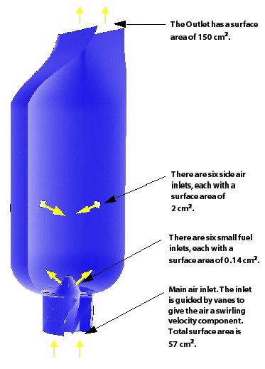
The can combustor is a feature of the gas turbine engine. Arranged around a central annulus, can combustors are designed to minimize emissions, burn very efficiently and keep wall temperatures as low as possible. This tutorial is designed to give a qualitative impression of the flow and temperature distributions inside a can combustor that burns methane in air. The basic geometry is shown below with a section of the outer wall cut away.
The simulation in this tutorial uses the Eddy Dissipation combustion model and the P1 radiation model.
Due to the fact that the fuel (methane) and oxidizer (air) undergo "fast" combustion (whereby the combustion rate is dominated by the rate of mixing of the materials), the Finite Rate Chemistry model is not a suitable combustion model for the combustor in this tutorial. The Combined EDM/FRC model capability is a superset of the Eddy Dissipation model capability, and has no benefit over the Eddy Dissipation model in this case. In fact, the convergence behavior of the Combined EDM/FRC model may be worse than that of the Eddy Dissipation model.
The Eddy Dissipation model is suitable for modeling "fast" combustion.
The Eddy Dissipation model tracks each individual chemical species (except for the constraint material) with its own transport equation. This model is flexible in that you can readily add new materials, such as additional fuels, to the simulation without complications. A limitation of this model is that radical or intermediate species, such as CO, cannot be calculated with adequate accuracy. This may lead to over-prediction of flame temperature, in particular in fuel-rich regions.
If this is the first tutorial you are working with, it is important to review the following topics before beginning:
Create a working directory.
Ansys CFX uses a working directory as the default location for loading and saving files for a particular session or project.
Download the
combustor.zipfile here .Unzip
combustor.zipto your working directory.Ensure that the following tutorial input file is in your working directory:
CombustorMesh.gtm
Set the working directory and start CFX-Pre.
For details, see Setting the Working Directory and Starting Ansys CFX in Stand-alone Mode.
You will first define a domain that includes a variable composition mixture. These mixtures are used to model combusting and reacting flows in CFX.
In CFX-Pre, select File > New Case.
Select General and click .
Select File > Save Case As.
Under File name, type
CombustorEDM.Click .
If prompted, click Overwrite.
Right-click
Meshand select Import Mesh > CFX Mesh.The Import Mesh dialog box appears.
Configure the following setting(s):
Setting
Value
File name
CombustorMesh.gtm
Click Open.
To enable combustion modeling, you must create a variable composition mixture.
In the Outline tree, right-click Materials and select Insert > Material.
Set the name to
Methane Air Mixtureand click .Configure the following setting(s):
Tab
Setting
Value
Basic Settings
Option
Reacting Mixture
Material Group
Gas Phase Combustion
Reactions List
Methane Air WD1 NO PDF [a]
Mixture Properties
Mixture Properties
(Selected)
Mixture Properties
> Radiation Properties
> Refractive Index
(Selected) [b]
Mixture Properties
> Radiation Properties
> Absorption Coefficient
(Selected)
Mixture Properties
> Radiation Properties
> Scattering Coefficient
(Selected)
The
Methane Air WD1 NO PDFreaction specifies complete combustion of the fuel into its products in a single-step reaction. The formation of NO is also modeled and occurs in an additional reaction step. Click Multi-select from extended list to display the
Reactions List dialog box,
then click Import Library
Data
to display the
Reactions List dialog box,
then click Import Library
Data
 and select the appropriate
reaction to import.
and select the appropriate
reaction to import.Setting the radiation properties explicitly will significantly shorten the solution time because the CFX-Solver will not have to calculate radiation mixture properties.
Click .
If Default Domain does not currently appear
under Flow Analysis 1 in the Outline tree:
Edit Case Options > General in the Outline tree view and ensure that Automatic Default Domain is turned on.
You now need to edit Default Domain so
that it is representative of the Eddy Dissipation combustion and P
1 radiation models.
Edit
Default Domainand configure the following setting(s):Tab
Setting
Value
Basic Settings
Location and Type
> Location
B152, B153, B154, B155, B156
Fluid and Particle Definitions
Fluid 1
Fluid and Particle Definitions
> Fluid 1
> Material
Methane Air Mixture
Domain Models
> Pressure
> Reference Pressure
1 [atm] [a]
Fluid Models
Heat Transfer
> Option
Thermal Energy
Turbulence
> Option
k-Epsilon
Combustion
> Option
Eddy Dissipation
Combustion
> Eddy Dissipation Model Coefficient B
(Selected)
Combustion
> Eddy Dissipation Model Coefficient B
> EDM Coeff. B
0.5 [b]
Thermal Radiation
> Option
P 1
Component Models
> Component
> N2
(Selected)
Component Models
> Component
> N2
> Option
Constraint
It is important to set a realistic reference pressure in this tutorial because the components of
Methane Air Mixtureare ideal gases.This includes a simple model for partial premixing effects by turning on the Product Limiter. When it is selected, nonzero initial values are required for the products. The products limiter is not recommended for multi-step eddy dissipation reactions, and so is set for this single step reaction only.
Click .
Create a new boundary by clicking Boundary
 and set the name to
 fuelin.Configure the following setting(s):
Tab
Setting
Value
Basic Settings
Boundary Type
Inlet
Location
fuelin
Boundary Details
Mass and Momentum
> Normal Speed
40 [m s^-1]
Heat Transfer
> Static Temperature
300 [K]
Component Details
> CH4
(Selected)
Component Details
> CH4
> Mass Fraction
1.0
Click .
Two separate boundary conditions will be applied for the incoming air. The first is at the base of the can combustor. The can combustor employs vanes downstream of the bottom air inlet to give the incoming air a swirling velocity.
Create a new boundary named
airin.Configure the following setting(s):
Tab
Setting
Value
Basic Settings
Boundary Type
Inlet
Location
airin
Boundary Details
Mass and Momentum
> Normal Speed
10 [m s^-1]
Heat Transfer
> Static Temperature
300 [K]
Component Details
> O2
(Selected)
Component Details
> O2
> Mass Fraction
0.232 [a]
Click .
The secondary air inlets are located on the side of the vessel and introduce extra air to aid combustion.
Create a new boundary named
secairin.Configure the following setting(s):
Tab
Setting
Value
Basic Settings
Boundary Type
Inlet
Location
secairin
Boundary Details
Mass and Momentum
> Normal Speed
6 [m s^-1]
Heat Transfer
> Static Temperature
300 [K]
Component Details
> O2
(Selected)
Component Details
> O2
> Mass Fraction
0.232 [a]
Click .
Create a new boundary named
out.Configure the following setting(s):
Tab
Setting
Value
Basic Settings
Boundary Type
Outlet
Location
out
Boundary Details
Mass and Momentum
> Option
Average Static Pressure
Mass and Momentum
> Relative Pressure
0 [Pa]
Click .
The vanes above the main air inlet are to be modeled as thin surfaces. To create a vane as a thin surface in CFX-Pre, you must specify a wall boundary on each side of the vanes.
You will first create a new region that contains one side of each of the eight vanes.
Create a new composite region by selecting Insert > Regions > Composite Region.
Set the name of the composite region to
Vane Surfaces.Configure the following setting(s):
Click .
Create another composite region named
Vane Surfaces Other Side.Configure the following setting(s):
Tab
Setting
Value
Basic Settings
Dimension (Filter)
2D
Region List
F129.153, F132.153, F136.154, F138.154, F141.155, F145.155, F147.156, F150.156
Click .
Create a new boundary named
vanes.Configure the following setting(s):
Tab
Setting
Value
Basic Settings
Boundary Type
Wall
Location
Vane Surfaces,Vane Surfaces Other SideClick .
The default boundary for any undefined surface in CFX-Pre is a no-slip, smooth, adiabatic wall.
For radiation purposes, the wall is assumed to be a perfectly absorbing and emitting surface (emissivity = 1).
The wall is non-catalytic, that is, it does not take part in the reaction.
Since this tutorial serves as a basic model, heat transfer through the wall is neglected. As a result, no further boundary conditions need to be defined.
Click Global Initialization
 .
.Configure the following setting(s):
Tab
Setting
Value
Global Settings
Initial Conditions
> Cartesian Velocity Components
> Option
Automatic with Value
Initial Conditions
> Cartesian Velocity Components
> U
0 [m s^-1]
Initial Conditions
> Cartesian Velocity Components
> V
0 [m s^-1]
Initial Conditions
> Cartesian Velocity Components
> W
5 [m s^-1]
Initial Conditions
> Component Details
> O2
(Selected)
Initial Conditions
> Component Details
> O2
> Option
Automatic with Value
Initial Conditions
> Component Details
> O2
> Mass Fraction
0.232 [a]
Initial Conditions
> Component Details
> CO2
(Selected)
Initial Conditions
> Component Details
> CO2
> Option
Automatic with Value
Initial Conditions
> Component Details
> CO2
> Mass Fraction
0.01
Initial Conditions
> Component Details
> H2O
(Selected)
Initial Conditions
> Component Details
> H2O
> Option
Automatic with Value
Initial Conditions
> Component Details
> H2O
> Mass Fraction
0.01
Click .
Click Solver Control
 .
.Configure the following setting(s):
Tab
Setting
Value
Basic Settings
Convergence Control
> Max. Iterations
100
Convergence Control
> Fluid Timescale Control
> Timescale Control
Physical Timescale
Convergence Control
> Fluid Timescale Control
> Physical Timescale
0.025 [s]
Click .
Click Define Run
 .
.Configure the following setting(s):
Setting
Value
File name
CombustorEDM.def
Click .
CFX-Solver Manager automatically starts and, on the Define Run dialog box, Solver Input File is set.
If using stand-alone mode, quit CFX-Pre, saving the simulation (
.cfx) file.
The CFX-Solver Manager will be launched after CFX-Pre saves the CFX-Solver input file. You will be able to obtain a solution to the CFD problem by following the instructions below.
Note: If a fine mesh is used for a formal quantitative analysis of the flow in the combustor, the solution time will be significantly longer than for the coarse mesh. You can run the simulation in parallel to reduce the solution time. For details, see Obtaining a Solution in Parallel.
Ensure that the Define Run dialog box is displayed.
Solver Input File should be set to
CombustorEDM.def.Click Start Run.
CFX-Solver runs and attempts to obtain a solution. At the end of the run, a dialog box is displayed stating that the simulation has ended.
Select Post-Process Results.
If using stand-alone mode, select Shut down CFX-Solver Manager.
Click .
When CFD-Post opens, experiment with the Edge Angle setting for the Wireframe object and the various
rotation and zoom features in order to place the geometry in a sensible
position. A setting of about 8.25 should result
in a detailed enough geometry for this exercise.
Right-click a blank area in the viewer and select Predefined Camera > View From +Y.
Create a new plane named
Plane 1.Configure the following setting(s):
Tab
Setting
Value
Geometry
Definition
> Method
ZX Plane
Color
Mode
Variable
Variable
Temperature
Click Apply.
The large area of high temperature through most of the vessel is due to forced convection.
In the next step you will color Plane 1 by the mass fraction of NO to view the distribution of NO within
the domain. The NO concentration is highest in the high temperature
region close to the outlet of the domain.
Modify the plane named
Plane 1.Configure the following setting(s):
Tab
Setting
Value
Color
Variable
NO.Mass Fraction
Click Apply.
Here you will change the color map (for Plane 1) to a grayscale map. The result will be a plot with different levels
of gray representing different mass fractions of NO. This technique
is especially useful for printing, to a black and white printer, any
image that contains a color map. Conversion to grayscale by conventional
means (that is, using graphics software, or letting the printer do
the conversion) will generally cause color legends to change to a
nonlinear distribution of levels of gray.
Modify the plane named
Plane 1.Configure the following setting(s):
Tab
Setting
Value
Color
Color Map
Inverse Greyscale
Click Apply.
In the next step, you will calculate the mass fraction of NO in the outlet stream.
Select Tools > Function Calculator or click the Calculators tab and select Function Calculator.
Configure the following setting(s):
Tab
Setting
Value
Function Calculator
Function
massFlowAve
Location
out
Variable
NO.Mass Fraction
Click Calculate.
A small amount of NO is released from the outlet of the combustor. This amount is lower than can normally be expected, and is mainly due to the coarse mesh and the short residence times in the combustor.
You will next look at the velocity vectors to show the flow field. You may notice a small recirculation in the center of the combustor. Running the problem with a finer mesh would show this region to be a larger recirculation zone. The coarseness of the mesh in this tutorial means that this region of flow is not accurately resolved.
On the Outline tab, under User Locations and Plots, clear the check box for Plane 1.
Plane 1is no longer visible.Create a new vector named
Vector 1.Configure the following setting(s):
Tab
Setting
Value
Geometry
Definition
> Locations
Plane 1
Symbol
Symbol Size
2
Click Apply.
Create a new plane named
Plane 2.Configure the following setting(s):
Tab
Setting
Value
Geometry
Definition
> Method
XY Plane
Definition
> Z
0.03 [m]
Plane Bounds
> Type
Rectangular
Plane Bounds
> X Size
0.5 [m]
Plane Bounds
> Y Size
0.5 [m]
Plane Type
> Sample
(Selected)
Plane Type
> X Samples
30
Plane Type
> Y Samples
30
Render
Show Faces
(Cleared)
Click Apply.
Modify
Vector 1.Configure the following setting(s):
Tab
Setting
Value
Geometry
Definition
> Locations
Plane 2
Click Apply.
To view the swirling velocity field, right-click in the viewer and select Predefined Camera > View From -Z.
You may also want to turn off the wireframe visibility. In the region near the fuel and air inlets, the swirl component of momentum (theta direction) results in increased mixing with the surrounding fluid in this region. As a result, more fuel is burned.