Chapter 21: Cavitation Around a Hydrofoil

This tutorial includes:

21.1. Tutorial Features

In this tutorial you will learn about:

Modeling flow with cavitation.
Using vector reduction in CFD-Post to clarify a vector plot with many arrows.
Importing and exporting data along a polyline.
Plotting computed and experimental results.

Component	Feature	Details
CFX-Pre	User Mode	General mode
	Analysis Type	Steady State
	Fluid Type	General Fluid
	Domain Type	Single Domain
	Turbulence Model	k-Epsilon
	Heat Transfer	Isothermal
	Multiphase
	Boundary Conditions	Inlet (Subsonic)
		Outlet (Subsonic)
		Symmetry Plane
		Wall: No-Slip
		Wall: Free-Slip
	Timestep	Physical Time Scale
CFX-Solver Manager	Restart
CFD-Post	Plots	Contour
		Line Locator
		Polyline
		Slice Plane
		Streamline
		Vector
	Other	Chart Creation
		Data Export
		Printing
		Title/Text
		Variable Details View

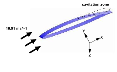
21.2. Overview of the Problem to Solve

This example demonstrates cavitation in the flow of water around a hydrofoil. A two-dimensional solution is obtained by modeling a thin slice of the hydrofoil and using two symmetry boundary conditions.

In this tutorial, an initial solution with no cavitation is generated to provide an accurate initial guess for a full cavitation solution, which is generated afterwards.

If this is the first tutorial you are working with, it is important to review the following topics before beginning:

21.3. Preparing the Working Directory

Create a working directory.
Ansys CFX uses a working directory as the default location for loading and saving files for a particular session or project.
Download the hydrofoil.zip file here .
Unzip hydrofoil.zip to your working directory.
Ensure that the following tutorial input files are in your working directory:
- HydrofoilExperimentalCp.csv
- HydrofoilGrid.def
Set the working directory and start CFX-Pre.
For details, see Setting the Working Directory and Starting Ansys CFX in Stand-alone Mode.

21.4. Simulating the Hydrofoil without Cavitation

This section describes the step-by-step definition of the flow physics in CFX-Pre.

21.4.1. Defining the Case Using CFX-Pre

In CFX-Pre, select File > New Case.
Select General and click OK.
Select File > Save Case As.
Under File name, type HydrofoilIni.
Click Save.

21.4.1.1. Importing the Mesh

Right-click Mesh and select Import Mesh > CFX-Solver Input.
The Import Mesh dialog box appears.
Configure the following setting(s):
Setting
Value
File name
HydrofoilGrid.def
Click Open.
Right-click a blank area in the viewer and select Predefined Camera > View From -Z.

Setting	Value
File name	HydrofoilGrid.def

21.4.1.2. Loading Materials

Since this tutorial uses Water Vapour at 25 C and Water at 25 C, you need to load these materials.

In the Outline tree view, right-click Materials and select Import Library Data.
The Select Library Data to Import dialog box is displayed.
Expand Water Data.
Select both Water Vapour at 25 C and Water at 25 C by holding Ctrl when selecting.
Click OK.

21.4.1.3. Creating the Domain

The fluid domain used for this simulation contains liquid water and water vapor. The volume fractions are initially set so that the domain is filled entirely with liquid.

Edit Case Options > General in the Outline tree view and ensure that Automatic Default Domain is turned on.
A domain named Default Domain should now appear under the Simulation > Flow Analysis 1 branch.
Double-click Default Domain.
Under Fluid and Particle Definitions, delete Fluid 1 and create a new fluid definition called Liquid Water.
Use the button to create another fluid named Water Vapor.

Configure the following setting(s):

Tab	Setting	Value
Basic Settings	Fluid and Particle Definitions	Liquid Water
Fluid and Particle Definitions > Liquid Water > Material	Water at 25 C ^[a]
Fluid and Particle Definitions	Water Vapor
Fluid and Particle Definitions > Water Vapor > Material	Water Vapour at 25 C ^[a]
Domain Models > Pressure > Reference Pressure	0 [atm]
Fluid Models	Multiphase > Homogeneous Model	(Selected)
Heat Transfer > Option	Isothermal
Heat Transfer > Fluid Temperature	300 [K]
Turbulence > Option	k-Epsilon
These two fluids have consistent reference enthalpies.

Tab

Setting

Value

Basic Settings

Fluid and Particle Definitions

Liquid Water

Fluid and Particle Definitions

> Liquid Water

> Material

Water at 25 C ^[a]

Fluid and Particle Definitions

Water Vapor

Fluid and Particle Definitions

> Water Vapor

> Material

Water Vapour at 25 C ^[a]

Domain Models

> Pressure

> Reference Pressure

0 [atm]

Fluid Models

Multiphase

> Homogeneous Model

(Selected)

Heat Transfer

> Option

Isothermal

Heat Transfer

> Fluid Temperature

300 [K]

Turbulence

> Option

k-Epsilon

These two fluids have consistent reference enthalpies.

Click OK.

21.4.1.4. Creating the Boundaries

The simulation requires inlet, outlet, wall and symmetry plane boundaries. The regions for these boundaries were imported with the grid file.

21.4.1.4.1. Inlet Boundary

Create a new boundary named Inlet.

Configure the following setting(s):

Tab	Setting	Value
Basic Settings	Boundary Type	Inlet
Basic Settings	Location	IN
Boundary Details	Mass And Momentum > Normal Speed	16.91 [m s^-1]
	Turbulence > Option	Intensity and Length Scale
	Turbulence > Fractional Intensity	0.03
	Turbulence > Eddy Length Scale	0.0076 [m]
Fluid Values	Boundary Conditions	Liquid Water
	Boundary Conditions > Liquid Water > Volume Fraction > Volume Fraction	1
	Boundary Conditions	Water Vapor
	Boundary Conditions > Water Vapor > Volume Fraction > Volume Fraction	0

Click OK.

21.4.1.4.2. Outlet Boundary

Create a new boundary named Outlet.
Configure the following setting(s):
Tab
Setting
Value
Basic Settings
Boundary Type
Outlet
Location
OUT
Boundary Details
Mass And Momentum
> Option

Static Pressure
Mass And Momentum
> Relative Pressure

51957 [Pa]
Click OK.

Tab	Setting	Value
Basic Settings	Boundary Type	Outlet
Location	OUT
Boundary Details	Mass And Momentum > Option	Static Pressure
Mass And Momentum > Relative Pressure	51957 [Pa]

21.4.1.4.3. Free Slip Wall Boundary

Create a new boundary named SlipWalls.
Configure the following setting(s):
Tab
Setting
Value
Basic Settings
Boundary Type
Wall
Location
BOT, TOP
Boundary Details
Mass And Momentum
> Option

Free Slip Wall
Click OK.

Tab	Setting	Value
Basic Settings	Boundary Type	Wall
Location	BOT, TOP
Boundary Details	Mass And Momentum > Option	Free Slip Wall

21.4.1.4.4. Symmetry Plane Boundaries

Create a new boundary named Sym1.
Configure the following setting(s):
Tab
Setting
Value
Basic Settings
Boundary Type
Symmetry
Location
SYM1
Click OK.

Tab	Setting	Value
Basic Settings	Boundary Type	Symmetry
Location	SYM1

Create a new boundary named Sym2.
Configure the following setting(s):
Tab
Setting
Value
Basic Settings
Boundary Type
Symmetry
Location
SYM2
Click OK.

Tab	Setting	Value
Basic Settings	Boundary Type	Symmetry
Location	SYM2

21.4.1.5. Setting Initial Values

Click Global Initialization .

Configure the following setting(s):

Tab	Setting	Value
Global Settings	Initial Conditions > Cartesian Velocity Components > Option	Automatic with Value
Initial Conditions > Cartesian Velocity Components > U	16.91 [m s^-1]
Initial Conditions > Cartesian Velocity Components > V	0 [m s^-1]
Initial Conditions > Cartesian Velocity Components > W	0 [m s^-1]
Fluid Settings	Fluid Specific Initialization	Liquid Water
Fluid Specific Initialization > Liquid Water > Initial Conditions > Volume Fraction > Option	Automatic with Value
Fluid Specific Initialization > Liquid Water > Initial Conditions > Volume Fraction > Volume Fraction	1
Fluid Specific Initialization	Water Vapor
Fluid Specific Initialization > Water Vapor > Initial Conditions > Volume Fraction > Option	Automatic with Value
Fluid Specific Initialization > Water Vapor > Initial Conditions > Volume Fraction > Volume Fraction	0

Tab

Setting

Value

Global Settings

Initial Conditions

> Cartesian Velocity Components

> Option

Automatic with Value

Initial Conditions

> Cartesian Velocity Components

> U

16.91 [m s^-1]

Initial Conditions

> Cartesian Velocity Components

> V

0 [m s^-1]

Initial Conditions

> Cartesian Velocity Components

> W

0 [m s^-1]

Fluid Settings

Fluid Specific Initialization

Liquid Water

Fluid Specific Initialization

> Liquid Water

> Initial Conditions

> Volume Fraction

> Option

Automatic with Value

Fluid Specific Initialization

> Liquid Water

> Initial Conditions

> Volume Fraction

> Volume Fraction

Fluid Specific Initialization

Water Vapor

Fluid Specific Initialization

> Water Vapor

> Initial Conditions

> Volume Fraction

> Option

Automatic with Value

Fluid Specific Initialization

> Water Vapor

> Initial Conditions

> Volume Fraction

> Volume Fraction

Click OK.

21.4.1.6. Setting Solver Control

Click Solver Control .

Configure the following setting(s):

Tab	Setting	Value
Basic Settings	Convergence Control > Max. Iterations	100
Convergence Control > Fluid Timescale Control > Timescale Control	Physical Timescale
Convergence Control > Fluid Timescale Control > Physical Timescale	0.01 [s]

Tab

Setting

Value

Basic Settings

Convergence Control

> Max. Iterations

100

Convergence Control

> Fluid Timescale Control

> Timescale Control

Physical Timescale

Convergence Control

> Fluid Timescale Control

> Physical Timescale

0.01 [s]

Note: For the Convergence Criteria, an RMS value of at least 1e-05 is usually required for adequate convergence, but the default value is sufficient for demonstration purposes.

Click OK.

21.4.1.7. Writing the CFX-Solver Input (.def) File

Click Define Run .
Configure the following setting(s):
Setting
Value
File name
HydrofoilIni.def
Click Save.
CFX-Solver Manager automatically starts and, on the Define Run dialog box, Solver Input File is set.
Quit CFX-Pre, saving the simulation (.cfx) file at your discretion.

Setting	Value
File name	HydrofoilIni.def

21.4.2. Obtaining the Solution using CFX-Solver Manager

While the calculations proceed, you can see residual output for various equations in both the text area and the plot area. Use the tabs to switch between different plots (for example, Momentum and Mass, Turbulence Quantities, and so on) in the plot area. You can view residual plots for the fluid and solid domains separately by editing the workspace properties.

Ensure that the Define Run dialog box is displayed.
Click Start Run.
CFX-Solver runs and attempts to obtain a solution. At the end of the run, a dialog box is displayed stating that the simulation has ended.
Select Post-Process Results.
If using stand-alone mode, select Shut down CFX-Solver Manager.
Click OK.

21.4.3. Viewing the Results Using CFD-Post

The following topics will be discussed:

21.4.3.1. Plotting Pressure Distribution Data

In this section, you will create a plot of the pressure coefficient distribution around the hydrofoil. The data will then be exported to a file for later comparison with data from the cavitating flow case, which will be run later in this tutorial.

Right-click a blank area in the viewer and select Predefined Camera > View From -Z.
Insert a new plane named Slice.
Configure the following setting(s):
Tab
Setting
Value
Geometry
Definition
> Method

XY Plane
Definition
> Z

5e-5 [m]
Render
Show Faces
(Cleared)
Click Apply.
Create a new polyline named Foil by selecting Insert > Location > Polyline from the main menu.
Configure the following setting(s):
Tab
Setting
Value
Geometry
Method
Boundary Intersection
Boundary List
Default Domain Default
Intersect With
Slice
Click Apply.
Zoom in on the center of the hydrofoil (near the cavity) to confirm the polyline wraps around the hydrofoil.

Tab	Setting	Value
Geometry	Definition > Method	XY Plane
Definition > Z	5e-5 [m]
Render	Show Faces	(Cleared)

Tab	Setting	Value
Geometry	Method	Boundary Intersection
Boundary List	Default Domain Default
Intersect With	Slice

Define the following expressions, remembering to click Apply after entering each definition:

Name	Definition
PCoef	(Pressure-51957[Pa])/(0.5996.2[kg m^-3]16.91[m s^-1]^2)
FoilChord	(X-minVal(X)@Foil)/(maxVal(X)@Foil-minVal(X)@Foil) ^[a]
This creates a normalized chord, measured in the X direction, ranging from 0 at the leading edge to 1 at the trailing edge of the hydrofoil.

Create a new variable named Pressure Coefficient.
Configure the following setting(s):
Setting
Value
Method
Expression
Scalar
(Selected)
Expression
PCoef
Click Apply.
Create a new variable named Chord.
Configure the following setting(s):
Setting
Value
Method
Expression
Scalar
(Selected)
Expression
FoilChord
Click Apply.
Note: Although the variables that were just created are only needed at points along the polyline, they exist throughout the domain.

Setting	Value
Method	Expression
Scalar	(Selected)
Expression	PCoef

Setting	Value
Method	Expression
Scalar	(Selected)
Expression	FoilChord

Now that the variables Chord and Pressure Coefficient exist, they can be associated with the previously defined polyline (the locator) to form a chart line. This chart line will be added to the chart object, which is created next.

Select Insert > Chart from the main menu.
Set the name to Pressure Coefficient Distribution.

Configure the following setting(s):

Tab	Setting	Value
General	Title	Pressure Coefficient Distribution
Data Series	Name	Solver Cp
Location	Foil
X Axis	Data Selection > Variable	Chord
Axis Range > Determine ranges automatically	(Cleared)
Axis Range > Min	0
Axis Range > Max	1
Axis Labels > Use data for axis labels	(Cleared)
Axis Labels > Custom Label	Normalized Chord Position
Y Axis	Data Selection > Variable	Pressure Coefficient
Axis Range > Determine Ranges Automatically	(Cleared)
Axis Range > Min	-0.5
Axis Range > Max	0.4
Axis Range > Invert Axis	(Selected)
Axis Labels > Use data for axis labels	(Cleared)
Axis Labels > Custom Label	Pressure Coefficient

Tab

Setting

Value

General

Title

Pressure Coefficient Distribution

Data Series

Name

Solver Cp

Location

Foil

X Axis

Data Selection

> Variable

Chord

Axis Range

> Determine ranges automatically

(Cleared)

Axis Range

> Min

Axis Range

> Max

Axis Labels

> Use data for axis labels

(Cleared)

Axis Labels

> Custom Label

Normalized Chord Position

Y Axis

Data Selection

> Variable

Pressure Coefficient

Axis Range

> Determine Ranges Automatically

(Cleared)

Axis Range

> Min

-0.5

Axis Range

> Max

0.4

Axis Range

> Invert Axis

(Selected)

Axis Labels

> Use data for axis labels

(Cleared)

Axis Labels

> Custom Label

Pressure Coefficient

Click Apply.
The chart appears in the Chart Viewer.

21.4.3.2. Exporting Pressure Distribution Data

You will now export the chord and pressure coefficient data along the polyline. This data will be imported and used in a chart later in this tutorial for comparison with the results for when cavitation is present.

Select File > Export > Export.
The Export dialog box appears
Configure the following setting(s):
Tab
Setting
Value
Options
File
NoCavCpData.csv
Locations
Foil
Export Geometry Information
(Selected) ^[a]
Select Variables
Chord, Pressure Coefficient
This causes X, Y, Z data to be included in the export file.
Click Save.
The file NoCavCpData.csv will be written in the working directory.

Tab	Setting	Value
Options	File	NoCavCpData.csv
Locations	Foil
Export Geometry Information	(Selected) ^[a]
Select Variables	Chord, Pressure Coefficient
This causes X, Y, Z data to be included in the export file.

21.4.3.3. Saving the Postprocessing State

If you are running CFD-Post in stand-alone mode, you will need to save the postprocessing state for use later in this tutorial, as follows:

Select File > Save State As.
Under File name type Cp_plot, then click Save.

In the next part of this tutorial, the solver will be run with cavitation turned on. Similar postprocessing follows, and the effect of cavitation on the pressure distribution around the hydrofoil will be illustrated in a chart.

21.5. Simulating the Hydrofoil with Cavitation

Earlier in this tutorial, you ran a simulation without cavitation. The solution from that simulation will serve as a starting point for the next simulation, which involves cavitation.

21.5.1. Defining the Case Using CFX-Pre

Ensure that the following tutorial input file is in your working directory:
- HydrofoilIni_001.res
Set the working directory and start CFX-Pre if it is not already running.
For details, see Setting the Working Directory and Starting Ansys CFX in Stand-alone Mode.
Select File > Open Case.
Select HydrofoilIni_001.res and click Open.
Save the case as Hydrofoil.cfx.

21.5.1.1. Adding Cavitation

Double-click Default Domain in the Outline tree view.

Configure the following setting(s):

Tab	Setting	Value
Fluid Pair Models	Fluid Pairs > Liquid Water \| Water Vapor > Mass Transfer > Option	Cavitation
Fluid Pairs > Liquid Water \| Water Vapor > Mass Transfer > Cavitation > Saturation Pressure	(Selected)
Fluid Pairs > Liquid Water \| Water Vapor > Mass Transfer > Cavitation > Saturation Pressure > Saturation Pressure	3574 [Pa] ^[a]
Saturation pressure can also be set by creating homogeneous binary mixtures, which are not used in this tutorial.

Tab

Setting

Value

Fluid Pair Models

Fluid Pairs

> Liquid Water | Water Vapor

> Mass Transfer

> Option

Cavitation

Fluid Pairs

> Liquid Water | Water Vapor

> Mass Transfer

> Cavitation

> Saturation Pressure

(Selected)

Fluid Pairs

> Liquid Water | Water Vapor

> Mass Transfer

> Cavitation

> Saturation Pressure

> Saturation Pressure

3574 [Pa] ^[a]

Saturation pressure can also be set by creating homogeneous binary mixtures, which are not used in this tutorial.

Click OK.

21.5.1.2. Modifying Solver Control

Click Solver Control .
Configure the following setting(s):
Tab
Setting
Value
Basic Settings
Convergence Control
> Max. Iterations

150 ^[a]
This allows up to 150 further iterations, when run as a restart.
Click OK.

Tab	Setting	Value
Basic Settings	Convergence Control > Max. Iterations	150 ^[a]
This allows up to 150 further iterations, when run as a restart.

21.5.1.3. Modifying Execution Control

Click Execution Control .

Configure the following setting(s):

Tab	Setting	Value
Run Definition	Input File Settings > Solver Input File	Hydrofoil.def ^[a]
You do not need to set the full path unless you are saving the solver file somewhere other than the working directory.

Tab

Setting

Value

Run Definition

Input File Settings

> Solver Input File

Hydrofoil.def ^[a]

You do not need to set the full path unless you are saving the solver file somewhere other than the working directory.

Confirm that the rest of the execution control settings are set appropriately.
Click OK.

21.5.1.4. Writing the CFX-Solver Input (.def) File

Click Define Run .
CFX-Solver Manager automatically starts and, on the Define Run dialog box, Solver Input File and the execution control settings are set.
If using stand-alone mode, quit CFX-Pre, saving the simulation (.cfx) file at your discretion.

21.5.2. Obtaining the Solution using CFX-Solver Manager

Ensure the Define Run dialog box is displayed.
Solver Input File should be set to Hydrofoil.def.

Configure the following setting(s) for the initial values file:

Tab	Setting	Value
Initial Values	Initial Values Specification	Selected
	Initial Values Specification > Initial Values	Initial Values 1
	Initial Values Specification > Initial Values > Initial Values 1 Settings > File Name ^[a]	`HydrofoilIni_001.res`
Click Browse and select the file from the working directory.

This is the solution from the starting-point run.

Click Start Run.
CFX-Solver runs and attempts to obtain a solution. At the end of the run, a dialog box is displayed stating that the simulation has ended.
Select Post-Process Results.
If using stand-alone mode, select Shut down CFX-Solver Manager.
Click OK.

21.5.3. Viewing the Results Using CFD-Post

You will restore the state file saved earlier in this tutorial while preventing the first solution (which has no cavitation) from loading. This will cause the plot of pressure distribution to use data from the currently loaded solution (which has cavitation). Data from the first solution will be added to the chart object by importing NoCavCpData.csv (the file that was exported earlier). A file containing experimental data will also be imported and added to the plot. The resulting chart will show all three sets of data (solver data with cavitation, solver data without cavitation, and experimental data).

Note: The experimental data is provided in HydrofoilExperimentalCp.csv which must be in your working directory before proceeding with this part of the tutorial.

Note: If using Ansys Workbench, CFD-Post will already be in the state in which you left it in the first part of this tutorial. In this case, proceed to step 5 below.

Select File > Load State.
Clear Load results.
Select Cp_plot.cst.
Click Open.
Click the Chart Viewer tab.
Edit Report > Pressure Coefficient Distribution.
Click the Data Series tab.
Configure the following setting(s):
Tab
Setting
Value
Data Series
Name
Solver Cp - with cavitation
This reflects the fact that the user-defined variable Pressure Coefficient is now based on the current results.
Click Apply.
You will now add the chart line from the first simulation.
Create a new polyline named NoCavCpPolyline.
Configure the following setting(s):
Tab
Setting
Value
Geometry
File
NoCavCpData.csv
Click Apply.
The data in the file is used to create a polyline with values of Pressure Coefficient and Chord stored at each point on it.
Edit Report > Pressure Coefficient Distribution.
Click the Data Series tab.
Click New .
Select Series 2 from the list box.

Tab	Setting	Value
Data Series	Name	Solver Cp - with cavitation

Tab	Setting	Value
Geometry	File	NoCavCpData.csv

Configure the following setting(s):

Tab	Setting	Value
Data Series	Name	Solver Cp - no cavitation
	Location	NoCavCpPolyline
	Custom Data Selection	(Selected)
	X Axis > Variable	Chord on NoCavCpPolyline
	Y Axis > Variable	Pressure Coefficient on NoCavCpPolyline

Click Apply.
The chart line (containing data from the first solution) is created, added to the chart object, and displayed in the Chart Viewer.
You will now add a chart line to show experimental results.
Click New .

Configure the following setting(s):

Tab	Setting	Value
Data Series	Name	Experimental Cp - with cavitation
Data Source > File	(Selected)
Data Source > File	HydrofoilExperimentalCp.csv
Line Display	Line Display > Line Style	Automatic
Line Display > Symbols	Rectangle

Tab

Setting

Value

Data Series

Name

Experimental Cp - with cavitation

Data Source

> File

(Selected)

Data Source

> File

HydrofoilExperimentalCp.csv

Line Display

> Line Style

Automatic

Line Display

> Symbols

Rectangle

Click Apply.
The chart line (containing experimental data) is created, added to the chart object, and displayed in the Chart Viewer.
If you want to save an image of the chart, select File > Save Picture from the main menu while the Chart Viewer is displayed. This will enable you to save the chart to an image file.
When you are finished, close CFD-Post.