


This tutorial includes:
Important: You must have the required Fortran compiler installed and set
in your system path in order to run this tutorial. For details on
which Fortran compiler is required for your platform, see the applicable
Ansys, Inc. installation guide. If you are not sure which Fortran
compiler is installed on your system, try running the cfx5mkext command (found in <CFXROOT>/bin
In this tutorial you will learn about:
Importing CEL expressions.
@REGION CEL syntax.
Setting up a user CEL function.
Setting up a monitor point to observe the temperature at a prescribed location.
Setting up an interface with conditional connection control.
Using the Monte Carlo radiation model with a directional source of radiation.
Postprocessing a transient simulation.
Component | Feature | Details |
|---|---|---|
CFX-Pre | User Mode | General mode |
Analysis Type | Transient | |
Fluid Type | General Fluid | |
Domain Type | Single Domain | |
Turbulence Model | k-Epsilon | |
Heat Transfer | Thermal Energy | |
Radiation | Monte Carlo | |
Buoyant Flow | ||
Boundary Conditions | Boundary Profile Visualization | |
Inlet (Profile) | ||
Outlet (Subsonic) | ||
Wall: No-Slip | ||
Wall: Adiabatic | ||
Wall: Fixed Temperature | ||
Domain Interface | Conditional GGI | |
Output Control | Transient Results Files | |
Monitor Points | ||
CEL (CFX Expression Language) | User CEL Function | |
CFD-Post | Plots | Animation |
Isosurface | ||
Point | ||
Slice Plane | ||
Other | Text Label with Auto Annotation | |
Changing the Color Range | ||
Legend | ||
Time Step Selection | ||
Transient Animation with Movie Generation |
This tutorial simulates a room with a thermostat-controlled air conditioner adjacent to a closet. The closet door is initially closed and opens during the simulation.
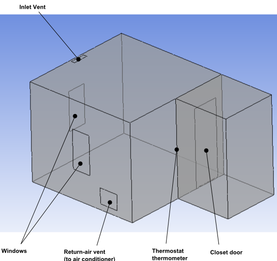
The thermostat switches the air conditioner on and off based on the following data:
A set point of 22°C (the temperature at or above which the air conditioner turns on)
A temperature tolerance of 1°C (the amount by which cooling continues below the set point before the air conditioner turns off)
The temperature at a wall-mounted thermometer
Air flows in steadily from an inlet vent on the ceiling, and flows out through a return-air vent near the floor. When the air conditioner is turned on, the incoming air temperature is reduced compared to the outgoing air temperature. When the air conditioner is turned off, the incoming air temperature is set equal to the outgoing air temperature.
Two windows enable sunlight to enter and heat the room. The walls (except for the closet door and part of the wall surrounding the closet door) and windows are assumed to be at a constant 26 °C. The simulation is transient, and continues long enough to enable the air conditioner to cycle on and off.
If this is the first tutorial you are working with, it is important to review the following topics before beginning:
Create a working directory.
Ansys CFX uses a working directory as the default location for loading and saving files for a particular session or project.
Download the
hvac.zipfile here .Unzip
hvac.zipto your working directory.Ensure that the following tutorial input files are in your working directory:
HVAC_expressions.cclHVACMesh.gtmTStat_Control.FNote: You must have a Fortran compiler installed on your system to perform this tutorial.
Set the working directory and start CFX-Pre.
For details, see Setting the Working Directory and Starting Ansys CFX in Stand-alone Mode.
In CFX-Pre, select File > New Case.
Select General and click .
Select File > Save Case As.
Under File name, type
HVAC.Click .
Right-click
Meshand select Import Mesh > CFX Mesh.The Import Mesh dialog box appears.
Configure the following setting(s):
Setting
Value
File name
HVACMesh.gtm
Click .
Right-click a blank area in the viewer and select Predefined Camera > Isometric View (Z up) from the shortcut menu.
This tutorial uses several CEL expressions to store parameters and to evaluate other quantities that are required by the simulation. Import all of the expressions from the provided file:
Select File > Import > CCL.
Ensure that Import Method is set to Append.
Select
HVAC_expressions.ccl, which should be in your working directory.Click .
The table below lists the expressions, along with the definition and information for each expression:
Expression Name | Expression Definition | Information |
|---|---|---|
ACOn | Thermostat Function(TSensor,TSet,TTol,atstep) | On/off status of the air conditioner (determined by calling a user CEL function with the thermometer temperature, thermostat set point, and temperature tolerance). |
Cool TempCalc | TVentOut - (HeatRemoved / (MassFlow * 1.004 [kJ kg^-1 K^-1 ])) | Temperature of air at the return-air vent (determined by a CEL function). |
Flowrate | 0.06 [m^3 s^-1] | Volumetric flow rate of air entering the room. |
HeatRemoved | 1000 [J s^-1] | Rate of thermal energy removal when the air conditioner is on. |
MassFlow | 1.185 [kg m^-3] * Flowrate | Mass flow rate of air entering the room. |
TIn | ACOn*CoolTempCalc+(1-ACOn)*TVentOut | Temperature of inlet vent air (a function of the air conditioner on/off status, return-air vent temperature, thermal energy removal rate, and mass flow rate). |
TSensor | probe(T)@Thermometer | Thermometer temperature (determined by a CEL function that gets temperature data from a monitor point). |
TSet | 22 [C] | Thermometer set point. |
TTol | 1 [K] | Temperature tolerance. |
TVentOut | areaAve(T)@REGION:VentOut | Temperature of outlet vent air. |
XCompInlet | 5*(x-0.05 [m]) / 1 [m] | Direction vector components for guiding the inlet vent air in a diverging manner as it enters the room. |
ZCompInlet | -1+XCompInlet | |
tStep | 3 [s] | Time step size. |
tTotal | 225 [s] | Total time. |
The CEL function that evaluates the thermometer temperature relies on a monitor point that you will create later in this tutorial.
The CEL expression for the air conditioner on/off status requires a compiled Fortran subroutine and a user CEL function that uses the subroutine. These are created next, starting with the compiled subroutine.
Note: The expression for the return-air vent temperature, TVentOut, makes use of @REGION CEL syntax, which indicates
the mesh region named VentOut, rather than a
boundary named VentOut.
A Fortran subroutine that simulates the thermostat is provided with the tutorial input files. Before the subroutine can be used, it must be compiled for your platform.
You can compile the subroutine at any time before running CFX-Solver.
The operation is performed at this point in the tutorial so that you
have a better understanding of the values you need to specify in CFX-Pre when
creating a User CEL Function. The cfx5mkext command is used to compile the subroutine as described below.
Ensure that file TStat_Control.F is in your working directory.
You can examine the contents of this file in any text editor to gain a better understanding of the subroutine it contains.
Select Tools > Command Editor.
Type the following command in the Command Editor dialog box (make sure you do not miss the semicolon at the end of the line):
! system ("cfx5mkext TStat_Control.F") == 0 or die "cfx5mkext failed";This is equivalent to executing the following at a command prompt:
cfx5mkext TStat_Control.F
The
!indicates that the following line is to be interpreted as power syntax and not CCL. Everything after the!symbol is processed as Perl commands.systemis a Perl function to run a system command.The "
== 0 or die" will cause an error message to be returned if, for some reason, there is an error in processing the command.
Click Process to compile the subroutine.
Note: You can use the
-doubleoption to compile the subroutine for use with double precision CFX-Solver executables. That is:cfx5mkext -double TStat_Control.F
A subdirectory will have been created in your working directory
whose name is system dependent (for example, on Linux it is named linux). This subdirectory contains the shared object library.
Note: If you are running problems in parallel over multiple
platforms then you will need to create these subdirectories using
the cfx5mkext command for each different platform.
You can view more details about the
cfx5mkextcommand by running:cfx5mkext -help
You can set a Library Name and Library Path using the
-nameand-destoptions respectively.If these are not specified, the default Library Name is that of your Fortran file and the default Library Path is your current working directory.
Close the Command Editor dialog box.
The expression for the air conditioner on/off status is named ACOn. This expression consists of a call to a user CEL
function, Thermostat Function, which must be
created.
Before you create the user CEL function, you will first create
a user routine that holds basic information about the compiled Fortran
subroutine. You will then create a user function, Thermostat
Function, so that it is associated with the user routine.
Create the user routine:
From the main menu, select Insert > Expressions, Functions and Variables > User Routine or click User Routine
 .
.Set the name to
Thermostat Routine.Configure the following setting(s):
Tab
Setting
Value
Basic Settings
Option
User CEL Function
Calling Name
ac_on [a] Library Name
TStat_Control [b]
Library Path
(Working Directory) [c]
This is the name of the subroutine within the Fortran file. Always use lower case letters for the calling name, even if the subroutine name in the Fortran file is in upper case.
This is the name passed to the
cfx5mkextcommand by the -name option. If the -name option is not specified, a default is used. The default is the Fortran file name without the.Fextension.
Click .
Create the user CEL function:
From the main menu, select Insert > Expressions, Functions and Variables > User Function or click User Function
 .
.Set the name to
Thermostat Function.Configure the following setting(s):
Click .
This is a transient simulation. The total time and time step
are specified by expressions that you imported earlier. Use these
expressions to set up the Analysis Type information:
Right-click
Analysis Typein the Outline tree view and select Edit.Configure the following setting(s):
Tab
Setting
Value
Basic Settings
Analysis Type
> Option
Transient
Analysis Type
> Time Duration
> Option
Total Time
Analysis Type
> Time Duration
> Total Time
tTotal
Analysis Type
> Time Steps
> Option
Timesteps
Analysis Type
> Time Steps
> Timesteps
tStep
Analysis Type
> Initial Time
> Option
Automatic with Value
Analysis Type
> Initial Time
> Time
0 [s]
Click .
The domain that models the room air should model buoyancy, given the expected temperature differences, air speeds, and the size and geometry of the room. The domain must model radiation, since directional radiation (representing sunlight) will be emitted from the windows.
Create the domain:
Edit
Case Options>Generalin the Outline tree view and ensure that Automatic Default Domain is turned on.A domain named
Default Domainshould appear under theSimulationbranch.Edit
Default Domainand configure the following setting(s):Tab
Setting
Value
Basic Settings
Location and Type
> Location
B54,B64
Fluid and Particle Definitions
Fluid 1
Fluid and Particle Definitions
> Fluid 1
> Material
Air Ideal Gas
Domain Models
> Pressure
> Reference Pressure
1 [atm]
Domain Models
> Buoyancy Model
> Option
Buoyant
Domain Models
> Buoyancy Model
> Gravity X Dirn.
0 [m s^-2]
Domain Models
> Buoyancy Model
> Gravity Y Dirn.
0 [m s^-2]
Domain Models
> Buoyancy Model
> Gravity Z Dirn.
-g
Domain Models
> Buoyancy Model
> Buoy. Ref. Density
1.2 [kg m^-3]
Fluid Models
Heat Transfer
> Option
Thermal Energy
Turbulence
> Option
k-Epsilon
Thermal Radiation
> Option
Monte Carlo
Thermal Radiation
> Number of Histories
100000
Click .
Note: When using a statistical radiation model like Monte Carlo, the results can usually be improved (at the expense of increased computational time) by increasing the number of histories.
In this section you will define several boundaries:
An inlet vent that injects air into the room.
A return-air vent that lets air leave the room.
Fixed-temperature windows that emit directed radiation.
Fixed-temperature walls.
Create a boundary for the inlet vent, using the previously-loaded expressions for mass flow rate, flow direction, and temperature:
Create a boundary named
Inlet.Configure the following setting(s):
Tab
Setting
Value
Basic Settings
Boundary Type
Inlet
Location
Inlet
Boundary Details
Mass and Momentum
> Option
Mass Flow Rate
Mass and Momentum
> Mass Flow Rate
MassFlow
Flow Direction
> Option
Cartesian Components
Flow Direction
> X Component
XCompInlet
Flow Direction
> Y Component
0
Flow Direction
> Z Component
ZCompInlet
Heat Transfer
> Option
Static Temperature
Heat Transfer
> Static Temperature
TIn
Plot Options
Boundary Vector
(Selected)
Boundary Vector
> Profile Vec. Comps.
Cartesian Components
Click .
The viewer shows the inlet velocity profile applied at the inlet, which uses the expressions
XCompInletandZCompInletto specify a diverging flow pattern.Note: Ignore the physics errors that appear. They will be fixed by setting up the rest of the simulation. The error concerning the expression
TInis due to a reference toThermometer, which does not yet exist. A monitor point namedThermometerwill be created later as part of the output control settings.
Create a boundary for the return-air vent, specifying a relative pressure of 0 Pa:
Create a boundary named
VentOut.Configure the following setting(s):
Tab
Setting
Value
Basic Settings
Boundary Type
Outlet
Location
VentOut
Boundary Details
Mass and Momentum
> Option
Average Static Pressure
Mass and Momentum
> Relative Pressure
0 [Pa]
Click .
To model sunlight entering the room, the windows are required to emit directional radiation. To approximate the effect of the outdoor air temperature, assume that the windows have a fixed temperature of 26°C.
Create a boundary for the windows using a fixed temperature of 26°C and apply a radiation source of 600 W m^-2 in the (1, 1, -1) direction:
Create a boundary named
Windows.Configure the following setting(s):
Tab
Setting
Value
Basic Settings
Boundary Type
Wall
Location
Window1,Window2
Boundary Details
Heat Transfer
> Option
Temperature
Heat Transfer
> Fixed Temperature
26 [C]
Sources
Boundary Source
(Selected)
Boundary Source
> Sources
(Selected)
Create a new radiation source item by clicking Add new item
 and accepting the default name.
Configure the following setting(s) of
Radiation Source 1:Setting
Value
Option
Directional Radiation Flux
Radiation Flux
600 [W m^-2]
Direction
> Option
Cartesian Components
Direction
> X Component
1
Direction
> Y Component
1
Direction
> Z Component
-1
Configure the following setting(s):
Tab
Setting
Value
Plot Options
Boundary Vector
(Selected)
Boundary Vector
> Profile Vec. Comps.
Cartesian Components in Radiation Source 1
Click .
The direction of the radiation is shown in the viewer.
The default boundary for any undefined surface in CFX-Pre is a no-slip, smooth, adiabatic wall. For this simulation, assume that the walls have a fixed temperature of 26°C. A more detailed simulation would model heat transfer through the walls.
For radiation purposes, assume that the default wall is a perfectly absorbing and emitting surface (emissivity = 1).
Set up the default wall boundary:
Edit the boundary named
Default Domain Default.Configure the following setting(s):
Tab
Setting
Value
Boundary Details
Heat Transfer
> Option
Temperature
Heat Transfer
> Fixed Temperature
26 [C]
Thermal Radiation
> Option
Opaque
Thermal Radiation
> Emissivity
1
Click .
Because this boundary is opaque with an emissivity of 1, all of the radiation is absorbed and none of the radiation is reflected. With no reflected radiation, the Diffuse Fraction setting has no effect. For lower values of emissivity, some radiation is reflected, and the Diffuse Fraction setting controls the fraction of the reflected radiation that is diffuse, with the remainder being specular (directional).
Click Domain Interface
 , set Name to
 ClosetWall, and click .Configure the following setting(s):
Tab
Setting
Value
Basic Settings
Interface Side 1
> Region List
F51.54
Interface Side 2
> Region List
F51.64
Additional Interface Models
Mass And Momentum
> Option
No Slip Wall
Heat Transfer
(Selected)
Heat Transfer
> Option
Conservative Interface Flux
Heat Transfer
> Interface Model
> Option
Thin Material
Heat Transfer
> Interface Model
> Material
Building Board Hardwood [a]
Heat Transfer
> Interface Model
> Thickness
12 [cm]
Thermal Radiation
(Selected)
Thermal Radiation
> Option
Opaque
Thermal Radiation
> Emissivity
1
Click the Ellipsis
 icon to open the Material dialog box. Click Import Library Data
  . In the Select Library Data to Import dialog box, select
 Building Board Hardwoodunder theCHT Solidsbranch and click . In the Material dialog box, selectBuilding Board Hardwoodunder theCHT Solidsbranch and click .
Click .
Create an expression named tOpen:
In the Outline tree view, expand Expressions, Functions and Variables, right-click Expressions and select Insert > Expression
Give the new expression the name:
tOpenIn the Definition area, type
t>150[s].Click Apply.
This expression will be used to indicate the point at which
the closet door is to open during the simulation. In the next section,
you will set up the door interface, and indicate that the interface
should change from closed to open when the expression tOpen evaluates to 1[] (true).
Create the interface:
Click Domain Interface
, set Name to ClosetDoor, and click .Configure the following settings:
Tab
Setting
Value
Basic Settings
Interface Side 1
> Region List
F53.54
Interface Side 2
> Region List
F53.64
Additional Interface Models
Mass And Momentum
> Option
Conservative Interface Flux
Conditional Connection Control
(Selected)
Conditional Connection Control
> Option
Irreversible State Change
Conditional Connection Control
> Logical Expression
tOpen
Conditional Connection Control
> Initial State
Closed
Click .
Next, set the properties of the closet door that will apply when the door is closed:
Edit the boundary named
ClosetDoor Side 1.Configure the following setting(s):
Tab
Setting
Value
Nonoverlap Conditions
Nonoverlap Conditions
(Selected)
Nonoverlap Conditions
> Boundary Type
Wall
Nonoverlap Conditions
> Mass and Momentum
> Option
No Slip Wall
Nonoverlap Conditions
> Heat Transfer
> Option
Adiabatic
Nonoverlap Conditions
> Thermal Radiation
> Option
Opaque
Nonoverlap Conditions
> Thermal Radiation
> Emissivity
1
Click .
Do the same for
ClosetDoor Side 2.
Create an interface under the closet door so that air can pass freely under the door. This connection will prevent the air in the closet from becoming isolated, so that the pressure level in the closet will be constrained.
Click Domain Interface
, set Name to DoorSpace, and click .Configure the following settings:
Tab
Setting
Value
Basic Settings
Interface Side 1
> Region List
F52.54
Interface Side 2
> Region List
F52.64
Click .
Click Global Initialization
 .
.Configure the following setting(s):
Tab
Setting
Value
Global Settings
Initial Conditions
> Velocity Type
Cartesian
Initial Conditions
> Cartesian Velocity Components
> Option
Automatic with Value
Initial Conditions
> Cartesian Velocity Components
> U
0 [m s^-1]
Initial Conditions
> Cartesian Velocity Components
> V
0 [m s^-1]
Initial Conditions
> Cartesian Velocity Components
> W
0 [m s^-1]
Initial Conditions
> Static Pressure
> Option
Automatic with Value
Initial Conditions
> Static Pressure
> Relative Pressure
0 [Pa]
Initial Conditions
> Temperature
> Option
Automatic with Value
Initial Conditions
> Temperature
> Temperature
21.8 [C]
Initial Conditions
> Turbulence
> Option
Intensity and Length Scale
Initial Conditions
> Turbulence
> Fractional Intensity
> Option
Automatic with Value
Initial Conditions
> Turbulence
> Fractional Intensity
> Value
0.05
Initial Conditions
> Turbulence
> Eddy Length Scale
> Option
Automatic with Value
Initial Conditions
> Turbulence
> Eddy Length Scale
> Value
0.25 [m]
Initial Conditions
> Radiation Intensity
> Option
Automatic with Value
Initial Conditions
> Radiation Intensity
> Blackbody Temperature
(Selected)
Initial Conditions
> Radiation Intensity
> Blackbody Temperature
> Blackbody Temp.
21.8 [C] [a]
Click .
In a typical transient simulation, there should be sufficient coefficient loops per time step to achieve convergence. In order to reduce the time required to run this particular simulation, reduce the maximum number of coefficient loops per time step to 3:
Click Solver Control
 .
.Configure the following setting(s):
Tab
Setting
Value
Basic Settings
Convergence Control
> Max. Coeff. Loops
3
Click .
Set up the solver to output transient results files that record pressure, radiation intensity, temperature, and velocity, on every time step:
Click Output Control
 .
.Click the Trn Results tab.
In the Transient Results list box, click Add new item
, set Name to Transient Results 1, and click .Configure the following setting(s) of
Transient
Results 1
:
To create the thermostat thermometer, set up a monitor point at the thermometer location. Also set up monitors to track the expressions for the temperature at the inlet, the temperature at the outlet, and the on/off status of the air conditioner.
Configure the following setting(s):
Tab
Setting
Value
Monitor
Monitor Objects
(Selected)
Create a new Monitor Points and Expressions item named
Thermometer.Configure the following setting(s) of
Thermometer:Setting
Value
Output Variables List
Temperature
Cartesian Coordinates
2.95, 1.5, 1.25
Create a new Monitor Points and Expressions item named
Temp at Inlet.Configure the following setting(s) of
Temp at Inlet:Setting
Value
Option
Expression
Expression Value
TIn
Create a new Monitor Points and Expressions item named
Temp at VentOut.Configure the following setting(s) of
Temp at VentOut:Setting
Value
Option
Expression
Expression Value
TVentOut
Create a new Monitor Points and Expressions item named
ACOnStatus.Configure the following setting(s) of
ACOnStatus:Setting
Value
Option
Expression
Expression Value
ACOn
Click .
Click Define Run
 .
.Configure the following setting(s):
Setting
Value
File name
HVAC.def
Click .
CFX-Solver Manager automatically starts and, on the Define Run dialog box, Solver Input File is set.
If using stand-alone mode, quit CFX-Pre, saving the simulation (
.cfx) file at your discretion.
When CFX-Pre has shut down and CFX-Solver Manager has started, start the solver and view the monitor points as the solution progresses:
Click Start Run.
After a few minutes, a User Points tab will appear.
On that tab, plots will appear showing the values of the monitor points:
ACOnStatusTemp at InletTemp at VentOutThermometer (Temperature)
Click one of the plot lines to see the value of the plot variable at that point.
It is difficult to see the plot values because all of the monitor points are plotted on the same scale. To see the plots in more detail, try displaying subsets of them as follows:
Right-click in the plot area and select Monitor Properties from the shortcut menu.
In the Monitor Properties dialog box, on the Plot Lines tab, expand the
USER POINTbranch in the tree.Clear the check boxes beside all of the monitor points except
ACOnStatus, then click Apply.Observe the plot for
ACOnStatus.You might have to move the dialog box out of the way to see the plot.
In the Monitor Properties dialog box, toggle each of the check boxes beside the monitor points, so that all of the monitor points are selected except for
ACOnStatus, then click Apply.Observe the plots for
Temp at Inlet,Temp at VentOut, andThermometer (Temperature).Click to close the Monitor Properties dialog box.
Select the check box next to Post-Process Results when the completion message appears at the end of the run.
If using stand-alone mode, select the check box next to Shut down CFX-Solver Manager.
Click .
You will first create some graphic objects to visualize the temperature distribution and the thermometer location. You will then create an animation to show how the temperature distribution changes.
In this section, you will create two planes and an isosurface of constant temperature, all colored by temperature. You will also create a color legend and a text label that reports the thermometer temperature.
In order to show the key features of the temperature distribution, create two planes colored by temperature as follows:
Load the res file (
HVAC_001.res) if you did not elect to load the results directly from CFX-Solver Manager.Right-click a blank area in the viewer, select Predefined Camera > Isometric View (Z up).
Create a ZX-Plane named
Plane 1with Y=2.25 [m]. Color it byTemperatureusing a user specified range from19 [C]to23 [C]. Turn off lighting (on the Render tab) so that the colors are accurate and can be interpreted properly using the legend.Create an XY plane named
Plane 2with Z=0.35 [m]. Color it using the same settings as for the first plane, and turn off lighting.
In order to show the plumes of cool air from the inlet vent, create a surface of constant temperature as follows:
Click Timestep Selector
 . The Timestep Selector dialog box appears.
Double-click the value: 69 s.
The time step is set to 69 s so that the cold air plume is visible.
Create an isosurface named
Cold Plumeas a surface ofTemperature= 19 °C.Color the isosurface by
Temperature(selectUse Plot Variable) and use the same color range as for the planes. Although the color of the isosurface will not show variation (by definition), it will be consistent with the coloration of the planes.On the Render tab for the isosurface, set Transparency to
0.5. Leave lighting turned on to help show the 3D shape of the isosurface.Click .
Note: The isosurface will not be visible in some time steps, but you will be able to see it when playing the animation (a step carried out later).
The legend title should not name the locator of any particular object since all objects are colored by the same variable and use the same range. Remove the locator name from the title and, in preparation for making an MPEG video later in this tutorial, increase the text size:
Edit
Default Legend View 1.On the Definition tab, change Title Mode to
Variable.This will remove the locator name from the legend.
Click the Appearance tab, then:
Change Precision to
2,Fixed.Change Text Height to
0.03.
Click .
In the next section, you will create a text label that displays
the value of the expression TSensor, which represents
the thermometer temperature. During the solver run, this expression
was evaluated using a monitor point named Thermometer. Although this monitor point data is stored in the results file,
it cannot be accessed. In order to support the expression for TSensor, create a point called Thermometer at the same location:
From the main menu, select Insert > Location > Point.
Set Name to
Thermometer.Set Point to
(2.95,1.5,1.25).Click the Color tab, then change Color to blue.
Click .
A marker appears at the thermometer location in the viewer. Note that you may have to rotate the results data to see the point.
Create a text label that shows the currently-selected time step and thermometer temperature.
Click Text
 .
.Accept the default name and click .
Configure the following setting(s):
Tab
Setting
Value
Definition
Text String
Time Elapsed:
(Selected) [a]
Type
Time Value
Click More to add a second line of text to the text object.
Configure the following setting(s):
Tab
Setting
Value
Definition
Text String (the second one)
Sensor Temperature:
Embed Auto Annotation
(Selected)
Type
Expression
Expression
TSensor
Appearance
Height
0.03
Click .
Ensure that the visibility for
Text 1is turned on.
The text label appears in the viewer, near the top.
Ensure that the view is set to Isometric View (Z up).
Click Timestep Selector
.Double-click the first time value (0 s).
Click Animation
 .
.The Animation dialog box appears.
Set Type to Keyframe Animation.
Click New
to create KeyframeNo1.Select
KeyframeNo1, then set # of Frames to200, then press Enter while in the # of Frames box.Tip: Be sure to press Enter and confirm that the new number appears in the list before continuing.
This will place 200 intermediate frames between the first and (yet to be created) second key frames, for a total of 202 frames. This will produce an animation lasting about 8.4 s since the frame rate will be 24 frames per second. Since there are 76 unique frames, each frame will be shown at least once.
Use the Timestep Selector to load the last time value (225 s).
In the Animation dialog box, click New
to create KeyframeNo2.The # of Frames parameter has no effect for the last keyframe, so leave it at the default value.
Click More Animation Options
 to expand the Animation dialog
box.
to expand the Animation dialog
box.Select Save Movie.
Set Format to
MPEG1.Specify a filename for the movie.
Click the Options button.
Change Image Size to
720
x 480
(or a similar resolution).Click the Advanced tab, and note the Quality setting. If your movie player cannot play the resulting MPEG, you can try using the Low or Custom quality settings.
Click .
Click To Beginning
 to rewind the active key frame to
 KeyframeNo1.Click Save animation state
 and save the animation to a file. This will enable
you to quickly restore the animation in case you want to make changes.
Animations are not restored by loading ordinary state files (those
with the .cst extension).
and save the animation to a file. This will enable
you to quickly restore the animation in case you want to make changes.
Animations are not restored by loading ordinary state files (those
with the .cst extension).Click Play the animation
 .
.If prompted to overwrite an existing movie, click Overwrite.
The animation plays and builds an
mpgfile.When you have finished, quit CFD-Post.
This tutorial uses an aggressive flow rate of air, a coarse mesh, large time steps, and a low cap on the maximum number of coefficient loops per time step. Running this tutorial with a flow rate of air that is closer to 5 changes of air per hour (0.03 m3 s-1), a finer mesh, smaller time steps, and a larger cap on the maximum number of coefficient loops, will produce more accurate results.
Running this simulation for a longer total time will allow you to see more on/off cycles of the air conditioner.