


This tutorial includes:
In this tutorial you will learn about:
Setting up a multiphase flow simulation involving air and water.
Using a fluid dependent turbulence model to set different turbulence options for each fluid.
Specifying buoyant flow.
Specifying a degassing outlet boundary to enable air, but not water, to escape from the boundary.
Using face culling in CFD-Post to turn off the visibility of one side of a surface.
Component | Feature | Details |
|---|---|---|
CFX-Pre | User Mode | General mode |
Analysis Type | Steady State | |
Fluid Type | General Fluid | |
Domain Type | Single Domain | |
Turbulence Model | Fluid Dependent | |
Dispersed Phase Zero Equation | ||
k-Epsilon | ||
Heat Transfer | None | |
Buoyant Flow | ||
Multiphase | ||
Boundary Conditions | Inlet (Subsonic) | |
Outlet (Degassing) | ||
Symmetry Plane | ||
Wall: (Slip Depends on Volume Fraction) | ||
Timestep | Physical Time Scale | |
CFD-Post | Plots | Default Locators |
Vector | ||
Other | Changing the Color Range | |
Symmetry |
This tutorial demonstrates the Eulerian-Eulerian multiphase model in CFX by simulating an airlift reactor. Airlift reactors are tall gas-liquid contacting vessels and are often used in processes where gas absorption is important (for example, bioreactors to dissolve oxygen in broths) and to limit the exposure of microorganisms to excessive shear imparted by mechanically driven mixers.
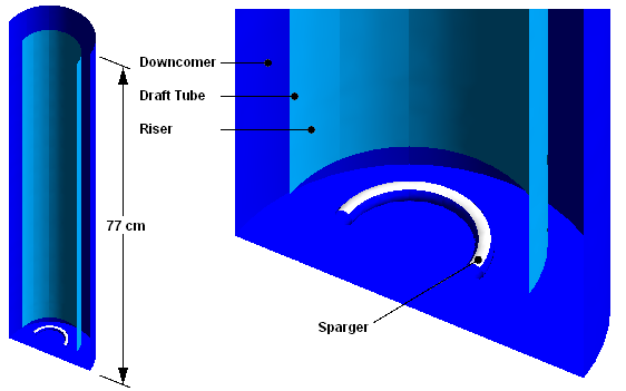
This tutorial models the dispersion of air bubbles in water. Air is supplied through a sparger at the bottom of the vessel and the rising action of the bubbles provides gentle agitation of the water. An internal tube (draft tube) directs recirculation of the flow. The airlift reactor is shown in a cut-away diagram in Figure 18.1: Cut-away Diagram of the Airlift Reactor.
Simple airlift reactors that are without a draft tube tend to develop irregular flow patterns and poor overall mixing. The draft tube in the airlift reactor helps to establish a regular flow pattern in the column and to achieve better uniformity in temperature, concentration, and pH in the liquid phase, but sometimes at the expense of decreased mass transfer from gas to liquid.
This tutorial also demonstrates the use of pairs of internal wall boundaries to model thin 3D features. In this case, a pair of wall boundaries is used to model the draft tube. Other applications include baffles and guide vanes. In the postprocessing section of this tutorial, you will learn how to use face culling to hide one side of a boundary. This technique enables you to independently color each boundary of a pair of back-to-back boundaries (located at the same position in 3D space, but with opposite orientation).
The airlift reactor that is modeled here is very similar to the laboratory bench scale prototype used by García-Calvo and Letón.
A formal analysis of this simulation involving a finer mesh is available at the end of this tutorial. For details, see Further Discussion.
If this is the first tutorial you are working with, it is important to review the following topics before beginning:
Create a working directory.
Ansys CFX uses a working directory as the default location for loading and saving files for a particular session or project.
Download the
bubble_column.zipfile here .Unzip
bubble_column.zipto your working directory.Ensure that the following tutorial input file is in your working directory:
BubbleColumnMesh.gtm
Set the working directory and start CFX-Pre.
For details, see Setting the Working Directory and Starting Ansys CFX in Stand-alone Mode.
In CFX-Pre, select File > New Case.
Select General and click .
Select File > Save Case As.
Under File name, type
BubbleColumn.Click .
Right-click
Meshand select Import Mesh > CFX Mesh.The Import Mesh dialog box appears.
Configure the following setting(s):
Setting
Value
File name
BubbleColumnMesh.gtm
Click Open.
Edit
Case Options>Generalin the Outline tree view and ensure that Automatic Default Domain is turned on. A domain namedDefault Domainshould now appear under theSimulationbranch.Double-click Default Domain.
In the Basic Settings tab, under Fluid and Particle Definitions, delete
Fluid
1
and create a new fluid definition calledAir.Use the
 button to create a new fluid named
 Water.Configure the following setting(s):
Tab
Setting
Value
Basic Settings
Location and Type
> Location
B1.P3, B2.P3
Fluid and Particle Definitions
Air
Fluid and Particle Definitions
> Air
> Material
Air at 25 C
Fluid and Particle Definitions
> Air
> Morphology
> Option
Dispersed Fluid
Fluid and Particle Definitions
> Air
> Morphology
> Mean Diameter
6 [mm]
Fluid and Particle Definitions
Water
Fluid and Particle Definitions
> Water
> Material
Water
Domain Models
> Pressure
> Reference Pressure
1 [atm]
Domain Models
> Buoyancy Model
> Option
Buoyant
Domain Models
> Buoyancy Model
> Gravity X Dirn.
0 [m s^-2]
Domain Models
> Buoyancy Model
> Gravity Y Dirn.
-9.81 [m s^-2]
Domain Models
> Buoyancy Model
> Gravity Z Dirn.
0 [m s^-2]
Domain Models
> Buoyancy Model
> Buoy. Ref. Density
997 [kg m^-3] [a]
Fluid Models
Multiphase
> Homogeneous Model
(Cleared) [b]
Multiphase
> Free Surface Model > Option
None
Heat Transfer
> Homogeneous Model
(Cleared)
Heat Transfer
> Option
Isothermal
Heat Transfer
> Fluid Temperature
25 [C]
Turbulence
> Homogeneous Model
(Cleared)
Turbulence
> Option
Fluid Dependent
Fluid Specific Models
Fluid
Water
Fluid
> Water
> Turbulence
> Option
k-Epsilon
Fluid Pair Models
Fluid Pair
Air | Water
Fluid Pair
> Air | Water
> Surface Tension Coefficient
(Selected)
Fluid Pair
> Air | Water
> Surface Tension Coefficient
> Surf. Tension Coeff.
0.072 [N m^-1] [c]
Fluid Pair
> Air | Water
> Momentum Transfer
> Drag Force
> Option
Grace
Fluid Pair
> Air | Water
> Momentum Transfer
> Drag Force
> Volume Fraction Correction Exponent
(Selected)
Fluid Pair
> Air | Water
> Momentum Transfer
> Drag Force
> Volume Fraction Correction Exponent
> Value
2 [d]
Fluid Pair
> Air | Water
> Momentum Transfer
> Non-drag forces
> Turbulent Dispersion Force
> Option
Favre Averaged Drag Force
Fluid Pair
> Air | Water
> Momentum Transfer
> Non-drag forces
> Turbulent Dispersion Force
> Dispersion Coeff.
1.0
Fluid Pair
> Air | Water
> Turbulence Transfer
> Option
Sato Enhanced Eddy Viscosity [e]
Click .
For this simulation of the airlift reactor, the required boundary conditions are:
An inlet for air on the sparger.
A degassing outlet for air at the liquid surface.
A pair of wall boundaries for the draft tube.
An exterior wall for the outer wall, base and sparger tube.
Symmetry planes.
At the sparger, create an inlet boundary that injects air at 0.3 m/s with a volume fraction of 0.25:
Create a new boundary named
Sparger.Configure the following setting(s):
Tab
Setting
Value
Basic Settings
Boundary Type
Inlet
Location
Sparger
Boundary Details
Mass And Momentum
> Option
Fluid Dependent
Fluid Values
Boundary Conditions
Air
Boundary Conditions
> Air
> Velocity
> Option
Normal Speed
Boundary Conditions
> Air
> Velocity
> Normal Speed
0.3 [m s^-1]
Boundary Conditions
> Air
> Volume Fraction
> Option
Value
Boundary Conditions
> Air
> Volume Fraction
> Volume Fraction
0.25
Boundary Conditions
Water
Boundary Conditions
> Water
> Velocity
> Option
Normal Speed
Boundary Conditions
> Water
> Velocity
> Normal Speed
0 [m s^-1]
Boundary Conditions
> Water
> Volume Fraction
> Option
Value
Boundary Conditions
> Water
> Volume Fraction
> Volume Fraction
0.75
Click .
Create a degassing outlet boundary at the top of the reactor:
Create a new boundary named
Top.Configure the following setting(s):
Tab
Setting
Value
Basic Settings
Boundary Type
Outlet
Location
Top
Boundary Details
Mass And Momentum
> Option
Degassing Condition
Click .
The draft tube is an infinitely thin surface that requires a wall boundary on both sides; if only one side has a boundary then CFX-Solver will fail.
The Free Slip condition can be used for
the gas phase since the contact area with the walls is near zero for
low gas phase volume fractions.
The required boundary settings are the same for both sides of the draft tube. From the point of view of solving the simulation, you could therefore define a single boundary and choose both sides of the tube as the location. However, the postprocessing section of this tutorial requires the use of separate boundaries in order to illustrate the use of face culling (a visualization technique), so you will create two wall boundaries instead.
Start by creating a wall boundary for the outer side of the draft tube:
Create a new boundary named
DraftTube Downcomer Side.Configure the following setting(s):
Tab
Setting
Value
Basic Settings
Boundary Type
Wall
Location
DraftTube
Boundary Details
Mass And Momentum
> Option
Fluid Dependent
Wall Roughness
> Option
Smooth Wall
Wall Contact Model
> Option
Use Volume Fraction
Fluid Values
Boundary Conditions
Air
Boundary Conditions
> Air
> Mass And Momentum
> Option
Free Slip Wall
Boundary Conditions
Water
Boundary Conditions
> Water
> Mass And Momentum
> Option
No Slip Wall
Click .
Now create a boundary named DraftTube Riser Side using the same settings, but located on F10.B1.P3 (the riser side of the draft tube).
To simulate the full geometry, create symmetry plane boundary
conditions on the Symmetry1 and Symmetry2 locators:
Create a new boundary named
SymP1.Configure the following setting(s):
Tab
Setting
Value
Basic Settings
Boundary Type
Symmetry
Location
Symmetry1
Click .
Create a new boundary named
SymP2.Configure the following setting(s):
Tab
Setting
Value
Basic Settings
Boundary Type
Symmetry
Location
Symmetry2
Click .
The remaining external regions are assigned to the default wall boundary. As for the draft tube boundary, set the air phase to use the free slip wall condition:
Edit
Default Domain Default.Configure the following setting(s):
Tab
Setting
Value
Boundary Details
Mass And Momentum
> Option
Fluid Dependent
Fluid Values
Boundary Conditions
Air
Boundary Conditions
> Air
> Mass And Momentum
> Option
Free Slip Wall
Boundary Conditions
Water
Boundary Conditions
> Water
> Mass And Momentum
> Option
No Slip Wall
Click .
The boundary specifications are now complete.
It often helps to set an initial velocity for a dispersed phase that is different to that of the continuous phase. This results in a nonzero drag between the phases that can help stability at the start of a simulation.
For some airlift reactor problems, improved convergence can be obtained by using CEL (CFX Expression Language) to specify a nonzero volume fraction for air in the riser portion and a value of zero in the downcomer portion. This should be done if two solutions are possible (for example, if the flow could go up the downcomer and down the riser).
Set the initial values:
Click Global Initialization
 .
.Since a single pressure field exists for a multiphase calculation, do not set pressure values on a per-fluid basis.
Configure the following setting(s):
Tab
Setting
Value
Fluid Settings
Fluid Specific Initialization
Air
Fluid Specific Initialization
> Air
> Initial Conditions
> Cartesian Velocity Components
> Option
Automatic with Value
Fluid Specific Initialization
> Air
> Initial Conditions
> Cartesian Velocity Components
> U
0 [m s^-1]
Fluid Specific Initialization
> Air
> Initial Conditions
> Cartesian Velocity Components
> V
0.3 [m s^-1]
Fluid Specific Initialization
> Air
> Initial Conditions
> Cartesian Velocity Components
> W
0 [m s^-1]
Fluid Specific Initialization
> Air
> Initial Conditions
> Volume Fraction
> Option
Automatic
Fluid Specific Initialization
Water [a]
Fluid Specific Initialization
> Water
> Initial Conditions
> Cartesian Velocity Components
> Option
Automatic with Value
Fluid Specific Initialization
> Water
> Initial Conditions
> Cartesian Velocity Components
> U
0 [m s^-1]
Fluid Specific Initialization
> Water
> Initial Conditions
> Cartesian Velocity Components
> V
0 [m s^-1]
Fluid Specific Initialization
> Water
> Initial Conditions
> Cartesian Velocity Components
> W
0 [m s^-1]
Fluid Specific Initialization
> Water
> Initial Conditions
> Volume Fraction
> Option
Automatic with Value
Fluid Specific Initialization
> Water
> Initial Conditions
> Volume Fraction
> Volume Fraction
1 [b]
Click .
Click Solver Control
 .
.Configure the following setting(s):
Tab
Setting
Value
Basic Settings
Advection Scheme
> Option
High Resolution
Convergence Control
> Max. Iterations
200
Convergence Control
> Fluid Timescale Control
> Timescale Control
Physical Timescale
Convergence Control
> Fluid Timescale Control
> Physical Timescale
1 [s]
Convergence Criteria
> Residual Type
MAX
Convergence Criteria
> Residual Target
1.0E-05 [a]
Convergence Criteria
> Conservation Target
(Selected)
Convergence Criteria
> Conservation Target
> Value
0.01
Advanced Options
Multiphase Control
(Selected)
Multiphase Control
> Volume Fraction Coupling
(Selected)
Multiphase Control
> Volume Fraction Coupling
> Option
Coupled [b]
Click .
Click Define Run
 .
.Configure the following setting(s):
Setting
Value
File name
BubbleColumn.def
Click .
CFX-Solver Manager automatically starts and, on the Define Run dialog box, Solver Input File is set.
If using stand-alone mode, quit CFX-Pre, saving the simulation (
.cfx) file at your discretion.
Start the simulation from CFX-Solver Manager:
Note: If you are using a fine mesh for a formal quantitative analysis of the flow in the reactor, the solution time will be significantly longer than for the coarse mesh. You can run the simulation in parallel to reduce the solution time. For details, see Obtaining a Solution in Parallel.
Ensure that the Define Run dialog box is displayed.
Click Start Run.
CFX-Solver runs and attempts to obtain a solution. This can take a long time depending on your system.
Select the check box next to Post-Process Results when the completion message appears at the end of the run.
If using stand-alone mode, select the check box next to Shut down CFX-Solver Manager.
Click .
You will first create plots of velocity and volume fraction. You will then display the entire geometry.
Because the simulation in this tutorial is conducted on a coarse grid, the results are only suitable for a qualitative demonstration of the multiphase capability of Ansys CFX.
The following topics will be discussed:
Right-click a blank area in the viewer and select Predefined Camera > View From -Z.
Create a new vector plot named
Vector 1.Configure the following setting(s):
Tab
Setting
Value
Geometry
Definition
> Locations
SymP1
Definition
> Variable
Water.Velocity
Color
Range
User Specified
Min
0 [m s^-1]
Max
1 [m s^-1]
Symbol
Symbol Size
0.3
Click Apply.
In the tree view, right-click
Vector 1, select Duplicate, and click OK to accept the default name,Vector 2.Edit
Vector 2.On the Geometry tab, set Definition > Variable to
Air.Velocityand click Apply.Compare
Vector 1andVector 2by toggling the visibility of each one.Zoom in as required.
Observe that the air flows upward, leaving the tank, at the degassing outlet.
Note that the air rises faster than the water in the riser and descends slower than the water in the downcomer.
Plot the volume fraction of air on the symmetry plane SymP1:
Right-click a blank area in the viewer and select Predefined Camera > View From -Z.
Turn on the visibility of
SymP1.Edit
SymP1.Configure the following setting(s) of
SymP1:Tab
Setting
Value
Color
Mode
Variable
Variable
Air.Volume Fraction
Range
User Specified
Min
0
Max
0.025
Click Apply.
Observe the volume fraction values throughout the domain.
Turn off the visibility of
SymP1.
Next, plot the volume fraction of air on each side of the draft tube:
Right-click a blank area in the viewer and select Predefined Camera > Isometric View (Y up).
Turn on the visibility of
DraftTube Downcomer Side.Modify
DraftTube Downcomer Sideby applying the following settings:Tab
Setting
Value
Color
Mode
Variable
Variable
Air.Volume Fraction
Range
User Specified
Min
0
Max
0.025
Click Apply.
Rotate the plot in the viewer to see both sides of
DraftTube Downcomer Side.Notice that the plot appears on both sides of the
DraftTube Downcomer Sideboundary. When viewing plots on internal surfaces, you must ensure that you are viewing the correct side. You will make use of the face culling rendering feature to turn off the visibility of the plot on the side of the boundary for which the plot does not apply.The
DraftTube Downcomer Sideboundary represents the side of the internal surface in the downcomer (in this case, outer) region of the reactor. To confirm this, you could make a vector plot of the variableNormal(representing the face normal vectors) on the locatorDraftTube Downcomer Side; the fluid is on the side opposite the normal vectors.In this case, you need to turn off the "front" faces of the plot; The front faces are, by definition, on the same side of the plot as the normal vectors.
Modify
DraftTube Downcomer Sideby applying the following settings:Tab
Setting
Value
Render
Show Faces
> Face Culling
Front Faces
Click Apply.
Rotate the image in the viewer to see the effect of face culling on
DraftTube Downcomer Side. You should see that the color appears on the downcomer side only.Turn on the visibility of
DraftTube Riser Side.Color the
DraftTube Riser Sideobject using the same color and rendering settings as forDraftTube Downcomer Side.The normal vectors for
DraftTube Riser Sidepoint opposite to those ofDraftTube Downcomer Side, so the faces onDraftTube Riser Sideare plotted only on the riser (in this case, inner) side of the airlift reactor.
Rotating the geometry will now correctly show the air volume fraction on each side of the draft tube.
Face culling was needed to prevent interference between the
plots on each side of the draft tube. To demonstrate this, try turning
off face culling for DraftTube Downcomer Side and watch the effect on the riser side. You might notice that the
plot from the downcomer side interferes with, or even completely overrides,
the riser-side plot. Results may vary, which is why face culling should
always be used to prevent possible interference.
Display the entire airlift reactor geometry by expanding User Locations and Plots and double-clicking the Default Transform object:
Configure the following setting(s) of
Default Transform:Tab
Setting
Value
Definition
Instancing Info From Domain
(Cleared)
Number of Graphical Instances
12
Apply Rotation
(Selected) Apply Rotation
> Method
Principal Axis
Apply Rotation
> Axis
Y
Apply Rotation
> Number of Passages
12
Click Apply.
A formal analysis of this airlift reactor was carried out on
a finer grid (having 21000+ nodes and a
maximum edge length of 0.005 m).
The analysis showed a region of air bubble recirculation at
the top of the reactor on the downcomer side. This was confirmed by
zooming in on a vector plot of Air.Velocity on SymP1 near the top of the downcomer. A similar plot of Water.Velocity revealed no recirculation of the water.
Other results of the simulation:
Due to their large
0.006m diameter, the air bubbles quickly attained a significant terminal slip velocity (that is, the terminal velocity relative to water). The resulting terminal slip velocity, obtained using the Grace drag model, is consistent with the prediction by Maneri and Mendelson and the prediction by Baker and Chao. These correlations predict a terminal slip velocity of about0.23m s-1 to0.25m s-1 for air bubbles of the diameter specified.The values of gas hold-up (the average volume fraction of air in the riser), the superficial gas velocity (the rising velocity, relative to the reactor vessel, of gas bubbles in the riser, multiplied by the gas hold-up), and the liquid velocity in the downcomer agree with the results reported by García-Calvo and Letón, for gas hold-up values of
0.03or less. At higher values of gas hold-up, the multifluid model does not account for pressure-volume work transferred from gas to liquid due to isothermal expansion of the bubbles. The simulation therefore tends to under-predict both the superficial gas velocity in the riser, and the liquid velocity in the downcomer for gas hold-up values greater than0.03.Note: Multiphase results files contain the vector variable
Fluid.Superficial Velocitydefined asFluid.Volume Fractionmultiplied byFluid.Velocity. This is sometimes also referred to as the fluid volume flux. The components of this vector variable are available as scalar variables (for example,Fluid.Superficial Velocity X).
Many reference texts on airlift reactors cite the Hughmark correlation as a standard for gas hold-up and superficial gas velocity in airlift reactors. However, the Hughmark correlation should not be used when liquid flow is concurrent with gas at velocities exceeding 0.1 m/s. In the airlift reactor described in this tutorial, the liquid velocity in the riser clearly exceeds 0.2 m/s, and the Hughmark correlation is therefore not applicable.