


This tutorial includes:
In this tutorial you will learn about:
Setting up a multiphase flow simulation involving air and water.
Importing meshes that have CFX-4 and CFX Mesh file formats.
Setting up a simulation using multiple frames of reference.
Using a fluid dependent turbulence model to set different turbulence options for each fluid.
Specifying buoyant flow.
Specifying a degassing outlet boundary to enable air, but not water, to escape from the boundary.
Connecting two domains (one for a tank and one for an impeller inside the tank) via Frozen Rotor interfaces.
Modeling rotational periodicity using periodic boundary conditions.
Using periodic GGI interfaces where the mesh does not match exactly.
Using thin surfaces for blade and baffle surfaces.
|
Component |
Feature |
Details |
|---|---|---|
|
CFX-Pre |
User Mode |
General mode |
|
Analysis Type |
Steady State | |
|
Fluid Type |
General Fluid | |
|
Domain Type |
Multiple Domain | |
|
Rotating Frame of Reference | ||
|
Turbulence Model |
Fluid Dependent | |
|
Dispersed Phase Zero Equation | ||
|
k-Epsilon | ||
|
Heat Transfer |
None | |
|
Buoyant Flow | ||
|
Multiphase | ||
|
Boundary Conditions |
Inlet (Subsonic) | |
|
Outlet (Degassing) | ||
|
Wall: Thin Surface | ||
|
Wall: (Slip Depends on Volume Fraction) | ||
|
Domain Interfaces |
Frozen Rotor | |
|
Periodic | ||
|
Thin Surface Partners | ||
|
Output Control | ||
|
Timestep |
Physical Time Scale | |
|
CFD-Post |
Plots |
Default Locators |
|
Slice Plane | ||
|
Other |
Quantitative Calculation |
This example simulates the mixing of water and air in a mixing vessel. The geometry consists of a mixing tank vessel, an air injection pipe, four baffles, a rotating impeller, and a shaft that runs vertically through the vessel. The impeller rotates at 84 rpm about the X axis (in the counterclockwise direction, when viewed from above). Air is injected into the vessel through an inlet pipe located below the impeller at a speed of 5 m/s. The inlet pipe diameter is 2.48 cm. Assume that both the water and air remain at a constant temperature of 25°C and that the air is incompressible, with a density equal to that at 25°C and 1 atmosphere. Also assume that the air bubbles are 3 mm in diameter.
Examine the steady-state distribution of air in the tank. Also calculate the torque and power required to turn the impeller at 84 rpm.
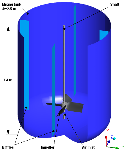
The figure above shows the full geometry with part of the tank walls and one baffle cut away. The symmetry of the vessel allows a 1/4 section of the full geometry to be modeled.
If this is the first tutorial you are working with, it is important to review the following topics before beginning:
Create a working directory.
Ansys CFX uses a working directory as the default location for loading and saving files for a particular session or project.
Download the
multiphase_mixer.zipfile here .Unzip
multiphase_mixer.zipto your working directory.Ensure that the following tutorial input files are in your working directory:
MixerImpellerMesh.gtmMixerTank.geo
Set the working directory and start CFX-Pre.
For details, see Setting the Working Directory and Starting Ansys CFX in Stand-alone Mode.
In CFX-Pre, select File > New Case.
Select General and click .
Select File > Save Case As.
Under File name, type
MultiphaseMixer.Click .
In this tutorial, two mesh files are provided: one for the mixer tank excluding the impeller, and one for the impeller. These meshes fit together to occupy the entire tank. The region occupied by the impeller mesh is indicated in Figure 17.2: Impeller Mesh Region.
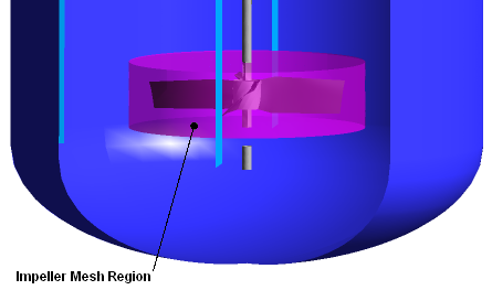
Next, you will import the mesh for the mixer tank, followed by the mesh for the impeller. The impeller mesh, as provided, is not located in the correct spatial position relative to the tank mesh. After importing the impeller mesh, you will move it to the correct position.
Note: This simulation involves the use of two domains: a stationary fluid domain on the main 3D region of the tank mesh and a rotating fluid domain on the main 3D region of the impeller mesh. It is not necessary to use separate meshes in this type of simulation, as long as there are 3D regions available for locating these two domains.
The mixer tank mesh is provided as a CFX-4 mesh file (*.geo). Import it as follows:
Right-click
Meshand select Import Mesh > Other.The Import Mesh dialog box appears.
Configure the following setting(s):
Setting
Value
Files of type
CFX-4 (*geo)
File name
MixerTank.geo
Options
> Mesh Units
m
Advanced Options
> CFX-4 Options
> Create 3D Regions on
> Fluid Regions (USER3D, POROUS)
(Cleared) [ a ]
Click Open.
The impeller mesh is provided as a CFX Mesh file (*.gtm). Import it as follows:
Right-click
Meshand select Import Mesh > CFX Mesh.The Import Mesh dialog box appears.
Configure the following setting(s):
Setting
Value
File name
MixerImpellerMesh.gtm
Click Open.
Right-click a blank area in the viewer and select Predefined Camera > Isometric View (X up) to view the mesh assemblies.
In the next step you will move the impeller mesh to its correct position.
Right-click
MixerImpellerMesh.gtmand select Transform Mesh.The Mesh Transformation Editor dialog box appears.
Configure the following setting(s):
Setting
Value
Transformation
Translation
Method
Deltas
Dx, Dy, Dz
0.275, 0, 0
Click Apply then Close.
You can now see the mesh on one of the periodic regions of the tank. To reduce the solution time for this tutorial, the mesh used is very coarse. This is not a suitable mesh to obtain accurate results, but it is sufficient for demonstration purposes.
Note: If you do not see the surface mesh, highlighting may be
turned off. If highlighting is disabled, toggle Highlighting  . The default highlight type will show the surface mesh for any selected
regions. If you see a different highlighting type, you can alter it
by selecting Edit > Options and browsing to CFX-Pre > Graphics
Style.
. The default highlight type will show the surface mesh for any selected
regions. If you see a different highlighting type, you can alter it
by selecting Edit > Options and browsing to CFX-Pre > Graphics
Style.
The mixer requires two domains: a rotating impeller domain and a stationary tank domain. Both domains contain water as a continuous phase and air as a dispersed phase. The domains will model turbulence, buoyancy, and forces between the fluids.
As stated in the problem description, the impeller rotates at 84 rpm.
Click Domain
 and
set the name to
and
set the name to impeller.Under the Fluid and Particle Definitions setting, delete
Fluid 1.Click Add new item
 and name it
 AirClick Add new item
and name it WaterConfigure the following setting(s):
Tab
Setting
Value
Basic Settings
Location and Type
> Location
Main
Fluid and Particle Definitions
Air
Fluid and Particle Definitions
> Air
> Material
Air at 25 C
Fluid and Particle Definitions
> Air
> Morphology
> Option
Dispersed Fluid
Fluid and Particle Definitions
> Air
> Morphology
> Mean Diameter
3 [mm]
Fluid and Particle Definitions
Water
Fluid and Particle Definitions
> Water
> Material
Water
Domain Models
> Pressure
> Reference Pressure
1 [atm]
Domain Models
> Buoyancy Model
> Option
Buoyant
Domain Models
> Buoyancy Model
> Gravity X Dirn.
-9.81 [m s^-2]
Domain Models
> Buoyancy Model
> Gravity Y Dirn.
0 [m s^-2]
Domain Models
> Buoyancy Model
> Gravity Z Dirn.
0 [m s^-2]
Domain Models
> Buoyancy Model
> Buoy. Ref. Density
997 [kg m^-3] [ a ]
Domain Models
> Domain Motion > Option
Rotating
Domain Models
> Domain Motion
> Angular Velocity
84 [rev min ^-1] [ b ]
Domain Models
> Domain Motion
> Axis Definition
> Rotation Axis
Global X
Fluid Models
Multiphase
> Homogeneous Model
(Cleared) [ c ]
Multiphase
> Free Surface Model > Option
None
Heat Transfer
> Homogeneous Model
(Cleared)
Heat Transfer
> Option
Isothermal
Heat Transfer
> Fluid Temperature
25 [C]
Turbulence
> Homogeneous Model
(Cleared)
Turbulence
> Option
Fluid Dependent
Fluid Specific Models
Fluid
Water
Fluid
> Water
> Turbulence
> Option
k-Epsilon
Fluid Pair Models
Fluid Pair
Air | Water
Fluid Pair
> Air | Water
> Surface Tension Coefficient
(Selected)
Fluid Pair
> Air | Water
> Surface Tension Coefficient
> Surf. Tension Coeff.
0.073 [N m^-1] [ d ]
Fluid Pair
> Air | Water
> Momentum Transfer
> Drag Force
> Option
Grace
Fluid Pair
> Air | Water
> Momentum Transfer
> Drag Force
> Volume Fraction Correction Exponent
(Selected)
Fluid Pair
> Air | Water
> Momentum Transfer
> Drag Force
> Volume Fraction Correction Exponent
> Value
4 [ e ]
Fluid Pair
> Air | Water
> Momentum Transfer
> Non-drag forces
> Turbulent Dispersion Force
> Option
Favre Averaged Drag Force
Fluid Pair
> Air | Water
> Momentum Transfer
> Non-drag forces
> Turbulent Dispersion Force
> Dispersion Coeff.
1
Fluid Pair
> Air | Water
> Turbulence Transfer
> Option
Sato Enhanced Eddy Viscosity [ f ]
Click .
Next, you will create a stationary domain for the main tank by copying the properties of the existing impeller domain.
Right-click
impellerand select Duplicate from the shortcut menu.Rename the duplicated domain to
tankand then open it for editing.Configure the following setting(s):
Tab
Setting
Value
Basic Settings
Location and Type
> Location
Primitive 3D
Domain Models
> Domain Motion
> Option
Stationary
Click .
The following boundary conditions will be set:
An inlet through which air enters the mixer.
A degassing outlet, so that only the gas phase can leave the domain.
Thin surfaces for the baffle.
A wall for the hub and the portion of the shaft that is in the rotating domain. This wall will be rotating, and therefore stationary relative to the rotating domain.
A wall for the portion of the shaft in the stationary domain. This wall will be rotating relative to the stationary domain.
When the default wall boundary is generated, the internal 2D regions of an imported mesh are ignored, while the regions that form domain boundaries are included.
Note: The blade surfaces of the impeller will be modeled using domain interfaces later in the tutorial.
Create a new boundary in the domain
tanknamedAirin.Configure the following setting(s):
Tab
Setting
Value
Basic Settings
Boundary Type
Inlet
Location
INLET_DIPTUBE
Boundary Details
Mass And Momentum
> Option
Fluid Dependent
Fluid Values
Boundary Conditions
Air
Boundary Conditions
> Air
> Velocity
> Option
Normal Speed
Boundary Conditions
> Air
> Velocity
> Normal Speed
5 [m s^-1]
Boundary Conditions
> Air
> Volume Fraction
> Option
Value
Boundary Conditions
> Air
> Volume Fraction
> Volume Fraction
1
Boundary Conditions
Water
Boundary Conditions
> Water
> Velocity
> Option
Normal Speed
Boundary Conditions
> Water
> Velocity
> Normal Speed
5 [m s^-1]
Boundary Conditions
> Water
> Volume Fraction
> Option
Value
Boundary Conditions
> Water
> Volume Fraction
> Volume Fraction
0
Click .
Create a degassing outlet to represent the free surface where air bubbles escape. The continuous phase (water) sees this boundary as a free-slip wall and does not leave the domain. The dispersed phase (air) sees this boundary as an outlet.
Create a new boundary in the domain
tanknamedLiquidSurface.Configure the following setting(s):
Tab
Setting
Value
Basic Settings
Boundary Type
Outlet
Location
WALL_LIQUID_SURFACE
Boundary Details
Mass And Momentum
> Option
Degassing Condition
Click .
Note that no pressure is specified for this boundary. The solver will compute a pressure distribution on this fixed-position boundary to represent the surface height variations that would occur in the real flow.
In CFX-Pre, thin surfaces can be created by specifying wall boundary conditions on both sides of internal 2D regions. Both sides of the baffle regions will be specified as walls in this case.
Create a new boundary in the domain
tanknamedBaffle.Configure the following setting(s):
Tab
Setting
Value
Basic Settings
Boundary Type
Wall
Location
WALL_BAFFLES [ a ]
Boundary Details
Mass And Momentum
> Option
Fluid Dependent
Wall Contact Model
> Option
Use Volume Fraction
Fluid Values
Boundary Conditions
Air
Boundary Conditions
> Air
> Mass and Momentum
> Option
Free Slip Wall [ b ]
Boundary Conditions
Water
Boundary Conditions
> Water
> Mass and Momentum
> Option
No Slip Wall
Click .
You will now set up a boundary for the portions of the shaft that are in the tank domain. Since the tank domain is not rotating, you need to specify a moving wall on the shaft to account for the shaft's rotation.
Part of the shaft is located directly above the air inlet, so the volume fraction of air in this location will be high and the assumption of zero contact area for the gas phase is not physically correct. In this case, a no slip boundary is more appropriate than a free slip condition for the air phase. When the volume fraction of air in contact with a wall is low, a free slip condition is more appropriate for the air phase.
In cases where it is important to correctly model the dispersed phase slip properties at walls for all volume fractions, you can declare both fluids as no slip, but set up an expression for the dispersed phase wall area fraction. The expression should result in an area fraction of zero for dispersed phase volume fractions from 0 to 0.3, for example, and then linearly increase to an area fraction of 1 as the volume fraction increases to 1.
Create a new boundary in the domain
tanknamedTankShaft.Configure the following setting(s):
Tab
Setting
Value
Basic Settings
Boundary Type
Wall
Location
WALL_SHAFT, WALL_SHAFT_CENTER
Boundary Details
Mass and Momentum
> Option
Fluid Dependent
Wall Contact Model
> Option
Use Volume Fraction
Fluid Values
Boundary Conditions
Air
Boundary Conditions
> Air
> Mass And Momentum
> Option
No Slip Wall
Boundary Conditions
> Air
> Mass And Momentum
> Wall Velocity
(Selected)
Boundary Conditions
> Air
> Mass And Momentum
> Wall Velocity > Option
Rotating Wall
Boundary Conditions
> Air
> Mass And Momentum
> Wall Velocity
> Angular Velocity
84 [rev min ^-1]
Boundary Conditions
> Air
> Mass And Momentum
> Wall Velocity
> Axis Definition
> Option
Coordinate Axis
Boundary Conditions
> Air
> Mass And Momentum
> Wall Velocity
> Axis Definition
> Rotation Axis
Global X
Select
Waterand set the same values as forAir.Click .
Create a new boundary in the domain
impellernamedHubShaft.Configure the following setting(s):
Tab
Setting
Value
Basic Settings
Boundary Type
Wall
Location
Hub,Shaft
Boundary Details
Mass And Momentum
> Option
Fluid Dependent
Wall Contact Model
> Option
Use Volume Fraction
Fluid Values
Boundary Conditions
Air
Boundary Conditions
> Air
> Mass And Momentum
> Option
Free Slip Wall
Boundary Conditions
Water
Boundary Conditions
> Water
> Mass and Momentum
> Option
No Slip Wall
Click .
As mentioned previously, when the volume fraction of air in contact with a wall is low, a free slip condition is more appropriate for the air phase.
In the tree view, open
tank Defaultfor editing.Configure the following setting(s):
Tab
Setting
Value
Boundary Details
Mass and Momentum
> Option
Fluid Dependent
Wall Contact Model
> Option
Use Volume Fraction
Fluid Values
Boundary Conditions
Air
Boundary Conditions
> Air
> Mass And Momentum
> Option
Free Slip Wall
Boundary Conditions
Water
Boundary Conditions
> Water
> Mass And Momentum
> Option
No Slip Wall
Click .
It is not necessary to set the default boundary in the impeller domain since the remaining surfaces will be assigned interface conditions in the next section.
The following interfaces will be set:
Blade thin surface interface.
Rotational periodic domain interfaces for the periodic faces of the tank and impeller.
Frozen Rotor interfaces between the impeller and tank domains.
You can model thin surfaces using either wall boundaries or domain interfaces. There are some differences between domain interfaces and ordinary wall boundaries; for example, CFX-Pre automatically detects the matching domain boundary regions when setting up a domain interface.
Previously, the thin surface representation of the tank baffle was modeled using boundary conditions. For demonstrational purposes, you will use a domain interface to model the thin surface representation of the impeller blade (even though using wall boundary conditions would also work).
Create a new domain interface named
Blade Thin Surface.Configure the following setting(s):
Tab
Setting
Value
Basic Settings
Interface Type
Fluid Fluid
Interface Side 1
> Domain (filter)
impeller
Interface Side 1
> Region List
Blade
Interface Side 2
> Domain (filter)
impeller
Interface Side 2
> Region List
Solid 3.3 2, Solid 3.6 2
Additional Interface Models
Mass And Momentum
> Option
Side Dependent [ a ]
Click .
Two boundaries named
Blade Thin Surface Side 1andBlade Thin Surface Side 2are created automatically.In the tree view, open
Blade Thin Surface Side 1for editing.Configure the following setting(s):
Tab
Setting
Value
Boundary Details
Mass and Momentum
> Option
Fluid Dependent
Wall Contact Model
> Option
Use Volume Fraction
Fluid Values
Boundary Conditions
Air
Boundary Conditions
> Air
> Mass And Momentum
> Option
Free Slip Wall
Boundary Conditions
Water
Boundary Conditions
> Water
> Mass And Momentum
> Option
No Slip Wall
Click .
In the tree view, open
Blade Thin Surface Side
2
for editing.Apply the same settings as for
Blade Thin Surface Side 1.Click .
Periodic domain interfaces can either be one-to-one or GGI interfaces.
One-to-one transformations occur for topologically similar meshes
whose nodes match within a given tolerance. One-to-one periodic interfaces
are more accurate and reduce CPU and memory requirements. Here, you
will choose the Automatic mesh connection method,
to let Ansys CFX choose between one-to-one and GGI.
Create a new domain interface named
ImpellerPeriodic.Configure the following setting(s):
Tab
Setting
Value
Basic Settings
Interface Type
Fluid Fluid
Interface Side 1
> Domain (Filter)
impeller
Interface Side 1
> Region List
Periodic1
Interface Side 2
> Domain (Filter)
impeller
Interface Side 2
> Region List
Periodic2
Interface Models
> Option
Rotational Periodicity
Interface Models
> Axis Definition
> Option
Coordinate Axis
Interface Models
> Axis Definition
> Rotation Axis
Global X
Mesh Connection
Mesh Connection Method
> Mesh Connection
> Option
Automatic
Click .
Create a new domain interface named
TankPeriodic.Configure the following setting(s):
Tab
Setting
Value
Basic Settings
Interface Type
Fluid Fluid
Interface Side 1
> Domain (Filter)
tank
Interface Side 1
> Region List
BLKBDY_TANK_PER1
Interface Side 2
> Domain (Filter)
tank
Interface Side 2
> Region List
BLKBDY_TANK_PER2
Interface Models
> Option
Rotational Periodicity
Interface Models
> Axis Definition
> Option
Coordinate Axis
Interface Models
> Axis Definition
> Rotation Axis
Global X
Mesh Connection
Mesh Connection Method
> Mesh Connection
> Option
Automatic
Click .
You will now create three Frozen Rotor interfaces for the regions connecting the two domains. In this case three separate interfaces are created. You should not try to create a single domain interface for multiple surfaces that lie in different planes.
Create a new domain interface named
Top.Configure the following setting(s):
Tab
Setting
Value
Basic Settings
Interface Type
Fluid Fluid
Interface Side 1
> Domain (Filter)
impeller
Interface Side 1
> Region List
Top
Interface Side 2
> Domain (Filter)
tank
Interface Side 2
> Region List
BLKBDY_TANK_TOP
Interface Models
> Option
General Connection
Interface Models
> Frame Change/Mixing Model
> Option
Frozen Rotor
Click .
Create a new domain interface named
Bottom.Configure the following setting(s):
Tab
Setting
Value
Basic Settings
Interface Type
Fluid Fluid
Interface Side 1
> Domain (Filter)
impeller
Interface Side 1
> Region List
Bottom
Interface Side 2
> Domain (Filter)
tank
Interface Side 2
> Region List
BLKBDY_TANK_BOT
Interface Models
> Option
General Connection
Interface Models
> Frame Change/Mixing Model
> Option
Frozen Rotor
Click .
Create a new domain interface named
Outer.Configure the following setting(s):
Tab
Setting
Value
Basic Settings
Interface Type
Fluid Fluid
Interface Side 1
> Domain (Filter)
impeller
Interface Side 1
> Region List
Outer
Interface Side 2
> Domain (Filter)
tank
Interface Side 2
> Region List
BLKBDY_TANK_OUTER
Interface Models
> Option
General Connection
Interface Models
> Frame Change/Mixing Model
> Option
Frozen Rotor
Click .
You will set the initial volume fraction of air to 0, and enable the initial volume fraction of water to be computed automatically. Since the volume fractions must sum to unity, the initial volume fraction of water will be 1.
It is important to understand how the velocity is initialized
in this tutorial. Here, both fluids use Automatic for the Cartesian Velocity Components option.
When the Automatic option is used, the initial
velocity field will be based on the velocity values set at inlets,
openings, and outlets. In this tutorial, the only boundary that has
a set velocity value is the inlet, which specifies a velocity of 5 [m s^-1]
for both phases. Without setting the Velocity Scale parameter, the resulting initial guess would be a uniform velocity
of 5 [m s^-1] in the X direction throughout
the domains for both phases. This is clearly not suitable since the
water phase is enclosed by the tank. When the boundary velocity conditions
are not representative of the expected domain velocities, the Velocity Scale parameter should be used to set a representative
domain velocity. In this case the velocity scale for water is set
to zero, causing the initial velocity for the water to be zero. The
velocity scale is not set for air, resulting in an initial velocity
of 5 [m s^-1] in the X direction for the
air. This should not be a problem since the initial volume fraction
of the air is zero everywhere.
Click Global Initialization
 .
.Configure the following setting(s):
Tab
Setting
Value
Fluid Settings
Fluid Specific Initialization
Air
Fluid Specific Initialization
> Air
> Initial Conditions
> Volume Fraction
> Option
Automatic with Value
Fluid Specific Initialization
> Air
> Initial Conditions
> Volume Fraction
> Volume Fraction
0
Fluid Specific Initialization
Water
Fluid Specific Initialization
> Water
> Initial Conditions
> Cartesian Velocity Components
> Option
Automatic
Fluid Specific Initialization
> Water
> Initial Conditions
> Cartesian Velocity Components
> Velocity Scale
(Selected)
Fluid Specific Initialization
> Water
> Initial Conditions
> Cartesian Velocity Components
> Velocity Scale
> Value
0 [m s^-1]
Click .
Generally, two different time scales exist for multiphase mixers.
The first is a small time scale based on the rotational speed of the
impeller, typically taken as 1 /  , resulting
in a time scale of 0.11 s for this case. The second time scale
is usually larger and based on the recirculation time of the continuous
phase in the mixer.
, resulting
in a time scale of 0.11 s for this case. The second time scale
is usually larger and based on the recirculation time of the continuous
phase in the mixer.
Using a time step based on the rotational speed of the impeller will be more robust, but convergence will be slow since it takes time for the flow field in the mixer to develop. Using a larger time step reduces the number of iterations required for the mixer flow field to develop, but reduces robustness. You will need to experiment to find an optimum time step.
Click Solver Control
 .
.Configure the following setting(s):
Tab
Setting
Value
Basic Settings
Advection Scheme
> Option
High Resolution
Convergence Control
> Max. Iterations
100
Convergence Control
> Fluid Timescale Control
> Timescale Control
Physical Timescale
Convergence Control
> Fluid Timescale Control
> Physical Timescale
1 [s] [ a ]
Convergence Criteria
(Default) [ b ]
Dynamic Model Control
Global Dynamic Model Control
(Selected)
Advanced Options
Multiphase Control
(Selected)
Multiphase Control
> Volume Fraction Coupling
(Selected)
Multiphase Control
> Volume Fraction Coupling
> Option
Coupled
Click .
You can monitor the value of an expression during the solver run so that you can view the volume fraction of air in the tank (the gas hold up). The gas hold up is often used to judge convergence in these types of simulations by converging until a steady-state value is achieved.
Create the following expressions:
TankAirHoldUp = volumeAve(Air.vf)@tank
ImpellerAirHoldUp = volumeAve(Air.vf)@impeller
TotalAirHoldUp = (volume()@tank * TankAirHoldUp +
                 volume()@impeller * ImpellerAirHoldUp) /
                 (volume()@tank + volume()@impeller)
Click Output Control
 .
.Configure the following setting(s):
Tab
Setting
Value
Monitor
Monitor Objects
(Selected)
Create a new Monitor Points and Expressions item named
Total Air Holdup.Configure the following setting(s) of
Total Air Holdup:Setting
Value
Option
Expression
Expression Value
TotalAirHoldUp
Click .
Click Define Run
 .
.Configure the following setting(s):
Setting
Value
File name
MultiphaseMixer.def
Click .
If you are notified the file already exists, click Overwrite.
Click .
If using stand-alone mode, quit CFX-Pre, saving the simulation (
.cfx) file at your discretion.
Start the simulation from CFX-Solver Manager:
Ensure that the Define Run dialog box is displayed.
Click Start Run.
CFX-Solver runs and attempts to obtain a solution. This can take a long time depending on your system.
Select the check box next to Post-Process Results when the completion message appears at the end of the run.
If using stand-alone mode, select the check box next to Shut down CFX-Solver Manager.
Click .
When CFD-Post starts, the Domain Selector dialog box might appear. If it does, ensure that both the impeller and tank domains are selected, then click to load the results from these domains. When the mixer geometry appears in the viewer, orient the view so that the X axis points up as follows:
Right-click a blank area in the viewer and select Predefined Camera > Isometric View (X up).
You will create some plots showing the distributions of velocity and other variables. You will also calculate the torque and power required to turn the impeller at 84 rpm.
Create a vertical plane that extends from the shaft to the tank wall at a location far from the baffle. This plane will be used as a locator for various plots, such as velocity vector plots and plots showing the distribution of air.
Create a new plane named
Plane 1.Configure the following setting(s):
Tab
Setting
Value
Geometry
Definition
> Method
Three Points
Definition
> Point 1
1, 0, 0
Definition
> Point 2
0, 1, -0.9
Definition
> Point 3
0, 0, 0
Click Apply.
Recall that the homogeneous multiphase option was not used when
specifying the domain settings (see the setting for Fluid Models > Multiphase
Options > Homogeneous Model in Rotating Domain for the Impeller). As a consequence, the air and water
velocity fields may differ from each other. Plot the velocity of water,
then air on Plane 1:
Create a new vector plot named
Vector 1.Configure the following setting(s):
Tab
Setting
Value
Geometry
Definition
> Locations
Plane 1
Variable
Water.Velocity in Stn Frame [ a ]
Symbol
Symbol Size
0.2
Normalize Symbols
(Selected)
Click Apply.
Turn off the visibility of
Plane 1to better see the vector plot.Observe the vector plot (in particular, near the top of the tank). Note that the water is not flowing out of the domain.
Change the variable to
Air.Velocity in Stn Frameand click Apply.Observe this vector plot, noting how the air moves upward all the way to the water surface, where it escapes.
Turn off the visibility of
Vector 1in preparation for the next plots.
Color Plane 1 to see the pressure distribution:
Turn on the visibility of
Plane 1.Configure the following setting(s) of
Plane 1:Tab
Setting
Value
Color
Mode
Variable
Variable
Pressure
Range
Local
Click Apply.
Note that the pressure field computed by the solver excludes the hydrostatic pressure corresponding to the specified buoyancy reference density. The pressure field including this hydrostatic component (as well as the reference pressure) can by visualized by plotting
Absolute
Pressure
.
To see the distribution of air, color Plane 1 by the volume fraction of air:
Configure the following setting(s) of
Plane 1:Tab
Setting
Value
Color
Mode
Variable
Variable
Air.Volume Fraction
Range
User Specified
Min
0
Max
0.04
Click Apply.
The user-specified range was made much narrower than the Global and Local ranges in order to better show the variation.
Areas of high shear strain rate or shear stress are typically also areas where the highest mixing occurs.
To see where the most of the mixing occurs, color Plane 1 by shear strain rate.
Configure the following setting(s) of
Plane 1:Tab
Setting
Value
Color
Variable
Air.Shear Strain Rate
Range
User Specified
Min
0 [s^-1]
Max
15 [s^-1]
Click Apply.
The user-specified range was made much narrower than the Global and Local ranges in order to better show the variation.
Modify the coloring of the
MultiphaseMixer_001>tank>tank Defaultobject by applying the following settings:Tab
Setting
Value
Color
Mode
Variable
Variable
Water.Wall Shear
Range
Local
Click Apply.
The legend for this plot shows the range of wall shear values.
The global maximum wall shear stress is much higher than the
maximum value on the default walls. The global maximum values occur
on the TankShaft boundary directly above the
inlet. Although these values are very high, the shear force exerted
on this boundary is small since the contact area fraction of water
is very small there.
Calculate the torque and power required to spin the impeller at 84 rpm:
Select Tools > Function Calculator from the main menu or click Function Calculator
 .
.Configure the following setting(s):
Tab
Setting
Value
Function Calculator
Function
torque
Location
Blade
Thin Surface Side 1
Axis
Global X
Fluid
All Fluids
Click Calculate to find the torque about the X axis imparted by both fluids on location
Blade Thin Surface Side 1.Repeat the calculation, setting Location to
Blade Thin Surface Side 2.
The sum of these two torques is approximately -72 [N m]
about the X axis. Multiplying by -4 to find the torque required by
all of the impeller blades gives a required torque of approximately
288 [N m] about the X axis. You could also include
the contributions from the locations HubShaft and TankShaft; however in this case their contributions
are negligible.
The power requirement is simply the required torque multiplied by the rotational speed (84 rpm = 8.8 rad/s): Power = 288 N m * 8.8 rad/s = 2534.4 W.
Remember that this value is the power requirement for the work done on the fluids; it does not account for any mechanical losses, motor efficiencies and so on. Also note that the accuracy of these results is significantly affected by the coarseness of the mesh. You should not use a mesh of this length scale to obtain accurate quantitative results.