


This tutorial includes:
In this tutorial you will learn about:
Creating and using a solid domain as a heating coil in CFX-Pre.
Creating a domain interface.
Modeling conjugate heat transfer in CFX-Pre.
Using electricity to power a heat source.
Plotting temperature on a cylindrical locator in CFD-Post.
Lighting in CFD-Post.
Component | Feature | Details |
|---|---|---|
CFX-Pre | User Mode | General mode |
Analysis Type | Steady State | |
Fluid Type | General Fluid | |
Domain Type | Multiple Domain | |
Turbulence Model | k-Epsilon | |
Shear Stress Transport | ||
Heat Transfer | Thermal Energy | |
Heat Transfer Modeling | Conjugate Heat Transfer (via Electrical Resistance Heating) | |
Boundary Conditions | Inlet (Subsonic) | |
Opening | ||
Wall: No-Slip | ||
Wall: Adiabatic | ||
CEL (CFX Expression Language) | ||
Timestep | Physical Time Scale | |
CFD-Post | Plots | Contour |
Cylindrical Locator | ||
Isosurface | ||
Temperature Profile Chart | ||
Other | Changing the Color Range | |
Expression Details View | ||
Lighting Adjustment | ||
Variable Details View | ||
Exporting Results to ANSYS |
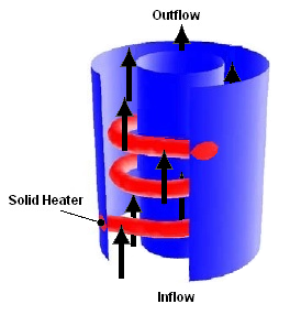
This tutorial demonstrates the capability of Ansys CFX to model conjugate heat transfer. In this tutorial, a heat exchanger is used to model the transfer of thermal energy from an electrically-heated solid copper coil to the water flowing around it.
There is a fluid domain for the water and a solid domain for the coil. The fluid domain is an annular region that envelops the coil, and has water at an initial temperature of 300 K flowing through it at 0.4 m/s. The copper coil has a 4.4 V difference in electric potential from one end to the other end and is given an initial temperature of 550 K. Assume that the copper has a uniform electrical conductivity of 59.6E+06 S/m and that there is a 1 mm thick calcium carbonate deposit on the heating coil.
The material parameters for the calcium carbonate deposit are:
Molar Mass =
100.087[kg kmol^-1]Density =
2.71[g cm^-3]Specific Heat Capacity =
0.9[J g^-1 K^-1]Thermal Conductivity =
3.85[W m^-1 K^-1]
If this is the first tutorial you are working with, it is important to review the following topics before beginning:
Create a working directory.
Ansys CFX uses a working directory as the default location for loading and saving files for a particular session or project.
Download the
cfx_heating_coil.zipfile here .Unzip
cfx_heating_coil.zipto your working directory.Ensure that the following tutorial input file is in your working directory:
HeatingCoilMesh.gtm
Set the working directory and start CFX-Pre.
For details, see Setting the Working Directory and Starting Ansys CFX in Stand-alone Mode.
In this tutorial, you will create a solid copper coil with a 1 mm thick calcium carbonate deposit.
In CFX-Pre, select File > New Case.
Select General and click .
Select File > Save Case As.
Under File name, type
HeatingCoil.If you are notified the file already exists, click Overwrite.
Click .
Right-click
Meshand select Import Mesh > CFX Mesh.The Import Mesh dialog box appears.
Configure the following setting(s):
Setting
Value
File name
HeatingCoilMesh.gtm
Click Open.
Right-click a blank area in the viewer and select Predefined Camera > Isometric View (Z up) from the shortcut menu.
Expand
Materialsin the tree view, right-clickCopperand select Edit.Configure the following setting(s) of
Copper:Tab
Setting
Value
Material Properties
Electromagnetic Properties
Expand the Electromagnetic Properties frame [a]
Electromagnetic Properties
> Electrical Conductivity
(Selected)
Electromagnetic Properties
> Electrical Conductivity
> Electrical Conductivity
59.6E+06 [S m^-1]
Click to apply these settings to
Copper.
Create a new material definition that will be used to model the calcium carbonate deposit on the heating coil:
Click Material
 and name the new material
 Calcium Carbonate.Configure the following setting(s):
Tab
Setting
Value
Basic Settings
Material Group
User [a]
Thermodynamic State
(Selected)
Thermodynamic State
> Thermodynamic State
Solid
Material Properties
Thermodynamic Properties
> Equation of State
> Molar Mass
100.087 [kg kmol^-1]
Thermodynamic Properties
> Equation of State
> Density
2.71 [g cm^-3] [b]
Thermodynamic Properties
> Specific Heat Capacity
(Selected)
Thermodynamic Properties
> Specific Heat Capacity
> Specific Heat Capacity
0.9 [J g^-1 K^-1] [b]
Transport Properties
> Thermal Conductivity
(Selected) [c]
Transport Properties
> Thermal Conductivity
> Thermal Conductivity
3.85 [W m^-1 K^-1]
The material properties for Calcium Carbonate defined in this table came directly from the Overview of the Problem to Solve section at the beginning of this tutorial.
You may need to first expand the Transport Properties frame by clicking Roll Down
 .
.
Click to apply these settings.
This simulation requires both a fluid domain and a solid domain. First, you will create a fluid domain for the annular region of the heat exchanger.
The fluid domain will include the region of fluid flow but exclude the solid copper heating coil.
Click Domain
 and
set the name to
and
set the name to WaterZone.Configure the following setting(s) of
WaterZone:Tab
Setting
Value
Basic Settings
Location and Type
> Location
Annulus [a]
Fluid and Particle Definitions
Fluid 1
Fluid and Particle Definitions
> Fluid 1
> Material
Water
Domain Models
> Pressure
> Reference Pressure
1 [atm]
Fluid Models
Heat Transfer
> Option
Thermal Energy
Turbulence
> Option
k-Epsilon
Initialization
Domain Initialization
(Selected)
Click to apply these settings to
WaterZone.
Since you know that the copper heating element will be much hotter than the fluid, you can initialize the temperature to a reasonable value. The initialization option that is set when creating a domain applies only to that domain.
Create the solid domain as follows:
Create a new domain named
SolidZone.Configure the following setting(s):
Tab
Setting
Value
Basic Settings
Location and Type
> Location
Coil [a]
Location and Type
> Domain Type
Solid Domain
Solid Definitions
Solid 1
Solid Definitions
> Solid 1
> Solid 1
> Material
Copper
Solid Models
Heat Transfer
> Option
Thermal Energy
Electromagnetic Model
(Selected)
Electromagnetic Model
> Electric Field Model
> Option
Electric Potential
Initialization
Domain Initialization
> Initial Conditions
> Temperature
> Option
Automatic with Value
Domain Initialization
> Initial Conditions
> Temperature
> Temperature
550 [K]
Click to apply these settings.
You will now set the boundary conditions using the values given in the problem description.
In order to pass electricity through the heating coil, you are going to specify a voltage of 0 [V] at one end of the coil and 4.4 [V] at the other end:
Click Boundary
 and select
 in SolidZonefrom the drop-down menu that appears.Name this new boundary
Groundand click .Configure the following setting(s):
Tab
Setting
Value
Basic Settings
Boundary Type
Wall
Location
Coil End 1[a]
Boundary Details
Electric Field
> Option
Voltage
Electric Field
> Voltage
0 [V]
Click to apply these settings.
Create a similar boundary named
Hotat the other end of the coil, Coil End 2, and apply a voltage of 4.4[V].

You will now create an inlet boundary for the cooling fluid (Water).
Create a new boundary in the
WaterZonedomain namedinflow.Configure the following setting(s):
Tab
Setting
Value
Basic Settings
Boundary Type
Inlet
Location
inflow
Boundary Details
Mass and Momentum
> Option
Normal Speed
Mass and Momentum
> Normal Speed
0.4 [m s^-1]
Heat Transfer
> Option
Static Temperature
Heat Transfer
> Static Temperature
300 [K]
Click to apply these settings.
An opening boundary is appropriate for the exit in this case because, at some stage during the solution, the coiled heating element will cause some recirculation at the exit. At an opening boundary you need to set the temperature of fluid that enters through the boundary. In this case it is useful to base this temperature on the fluid temperature at the outlet, since you expect the fluid to be flowing mostly out through this opening.
Insert a new expression by clicking Expression
 .
.Name this new expression
OutletTemperatureand press the Enter key to continue.In the Definition entry box, type the formula
areaAve(T)@outflowClick Apply.
Close the Expressions view by clicking Close
 at the top of the tree view.
Create a new boundary in the
WaterZonedomain namedoutflow.Configure the following setting(s):
Tab
Setting
Value
Basic Settings
Boundary Type
Opening
Location
outflow
Boundary Details
Mass and Momentum
> Option
Opening Pres. and Dirn
Mass and Momentum
> Relative Pressure
0 [Pa]
Heat Transfer
> Option
Static Temperature
Heat Transfer
> Static Temperature
OutletTemperature [a]
Click to apply these settings.
A default no slip, adiabatic wall boundary named WaterZone
Default will be applied automatically to the remaining
unspecified external boundaries of the WaterZone domain.
Two more boundary conditions are generated automatically when a domain interface is created to connect the fluid and solid domains. The domain interface is discussed in the next section.
Click Domain Interface
 from the row of icons located along
the top of the screen.
from the row of icons located along
the top of the screen.Accept the default name
Domain Interface 1by clicking .Configure the following setting(s) of
Domain Interface 1:Tab
Setting
Value
Basic Settings
Interface Type
Fluid Solid
Interface Side 1
> Domain (Filter)
WaterZone
Interface Side 1
> Region List
coil surface
Interface Side 2
> Domain (Filter)
SolidZone
Interface Side 2
> Region List
F22.33, F30.33, F31.33, F32.33, F34.33, F35.33
Additional Interface Models
Heat Transfer
(Selected)
Heat Transfer
> Interface Model
> Option
Thin Material
Heat Transfer
> Interface Model
> Material
Calcium Carbonate
Heat Transfer
> Interface Model
> Thickness
1 [mm] [a]
Click to apply these settings.
Click Solver Control
 .
.Configure the following setting(s):
Tab
Setting
Value
Basic Settings
Convergence Control
> Fluid Timescale Control
> Timescale Control
Physical Timescale
Convergence Control
> Fluid Timescale Control
> Physical Timescale
2 [s]
For the Convergence Criteria, an RMS value of at least 1e-05 is usually required for adequate convergence, but the default value is sufficient for demonstration purposes.
Click to apply these settings.
Click Define Run
 .
.Configure the following setting(s):
Setting
Value
File name
HeatingCoil.def
Click .
CFX-Solver Manager automatically starts and, on the Define Run dialog box, Solver Input File is set.
If using stand-alone mode, quit CFX-Pre, saving the simulation (
.cfx) file at your discretion.
Ensure that the Define Run dialog box is displayed.
Click Start Run.
CFX-Solver runs and attempts to obtain a solution. At the end of the run, a dialog box is displayed stating that the simulation has ended.
While the calculations proceed, you can see residual output for various equations in both the text area and the plot area. Use the tabs to switch between different plots (for example, Heat Transfer, Turbulence (KE), and so on) in the plot area. You can view residual plots for the fluid and solid domains separately by editing the workspace properties (under Workspace > Workspace Properties).
Select Post-Process Results.
If using stand-alone mode, select Shut down CFX-Solver Manager.
Click .
The following topics will be discussed:
To grasp the effect of the calcium carbonate deposit, it is beneficial to compare the temperature range on either side of the deposit.
When CFD-Post opens, if you see the Domain Selector dialog box, ensure that both domains are selected, then click OK.
Create a new contour named
Contour 1.Configure the following setting(s):
Click Apply.
Take note of the temperature range displayed below the Range drop-down box. The temperature on the outer surface of the deposit should range from around 380 [K] to 740 [K].
Change the contour location to
Domain Interface
1 Side 2
(the deposit side that is in contact with the coil) and click Apply.Notice how the temperature ranges from around 420 [K] to 815 [K] on the inner surface of the deposit.
Next, you will create a cylindrical locator close to the outside wall of the annular domain. This can be done by using an expression to specify radius and locating a particular radius with an isosurface.
Create a new expression by clicking Expression
.Set the name of this new expression to
expradiusand press the Enter key to continue.Configure the following setting(s):
Setting
Value
Definition
(x^2 + y^2)^0.5
Click Apply.
Create a new variable by clicking Variable
 .
.Set the name of this new variable to
radiusand press the Enter key to continue.Configure the following setting(s):
Setting
Value
Expression
expradius
Click Apply.
Insert a new isosurface by clicking Location
 > Isosurface.
Accept the default name
Isosurface 1by clicking .Configure the following setting(s):
Click Apply.
Turn off the visibility of
Contour 1so that you have an unobstructed view ofIsosurface 1.
Note: The default range legend now displayed is that of the isosurface and not the contour. The default legend is set according to what is being edited in the details view.
For a quantitative analysis of the temperature variation through the water and heating coil, it is beneficial to create a temperature profile chart.
First, you will create a line that passes through two turns of the heating coil. You can then graphically analyze the temperature variance along that line by creating a temperature chart.
Insert a line by clicking Location
> Line.Accept the default name
Line 1by clicking .Configure the following setting(s) of
Line 1Tab
Setting
Value
Geometry
Definition
> Point 1
-0.75, 0, 0
Definition
> Point 2
-0.75, 0, 2.25
Line Type
> Sample
(Selected)
Line Type
> Samples
200
Click Apply.
Create a new chart by clicking Chart
 .
.Name this chart
Temperature Profileand press the Enter key to continue.Click the Data Series tab.
Set Data Source > Location to
Line 1.Click the Y Axis tab.
Set Data Selection > Variable to
Temperature.Click Apply.
You can see from the chart that the temperature spikes upward when entering the deposit region and is at its maximum at the center of the coil turns.
Specular lighting is on by default. Specular lighting allows glaring bright spots on the surface of an object, depending on the orientation of the surface and the position of the light. You can disable specular lighting as follows:
Click the 3D Viewer tab at the bottom of the viewing pane.
Edit
Isosurface 1in the Outline tree view.Tab
Setting
Value
Render
Show Faces
> Specular
(Cleared)
Click Apply.
To move the light source, click within the 3D Viewer, then press and hold Shift while pressing the arrow keys left, right, up or down.
Tip: If using the stand-alone version, you can move the light source by positioning the mouse pointer in the viewer, holding down the Ctrl key, and dragging using the right mouse button.