


DesignXplorer is a Workbench component that you can use to examine the effect of changing parameters in a system. In this tutorial, two streams of water at different temperatures are mixed in a static mixer. You will see how changing the geometry and inlet flow rate affects the mixing effectiveness, as measured by the range of temperature over the outlet.
This tutorial includes:
- 5.1. Tutorial Features
- 5.2. Overview of the Problem to Solve
- 5.3. Setting Up Ansys Workbench
- 5.4. Creating the Project
- 5.5. Creating the Geometry in DesignModeler
- 5.6. Creating the Mesh
- 5.7. Setting up the Case with CFX-Pre
- 5.8. Setting the Output Parameter in CFD-Post
- 5.9. Investigating the Impact of Changing Design Parameters Manually
- 5.10. Using Design of Experiments
- 5.11. Viewing the Response Surface
- 5.12. Optimization based on the Response Surface
Note: Some of the instructions in this tutorial assume that you have sufficient licensing to have multiple applications open. If you do not have sufficient licensing, you may not be able to keep as many of the applications open as this tutorial suggests. In this case, simply close the applications as you finish with them.
In this tutorial you will learn about:
Creating a geometry in DesignModeler and creating a mesh.
Using General mode in CFX-Pre to set up a problem.
Using design points to manually vary characteristics of the problem to see how you can improve the mixing.
Using DesignXplorer to vary characteristics of the problem programmatically to find an optimal design.
Component | Feature | Details |
|---|---|---|
DesignModeler | Geometry Creation | |
Named Selections | ||
Meshing Application | Mesh Creation | |
CFX-Pre | User Mode | General mode |
Analysis Type | Steady State | |
Fluid Type | General Fluid | |
Domain Type | Single Domain | |
Turbulence Model | k-Epsilon | |
Heat Transfer | Thermal Energy | |
Boundary Conditions | Inlet (Subsonic) | |
Outlet (Subsonic) | ||
Wall: No-Slip | ||
Wall: Adiabatic | ||
Timescale | Physical Timescale | |
Expressions | Workbench input parameter | |
CFD-Post | Expressions | Workbench output parameter |
Parameters | Design Points | Manual changes |
DesignXplorer | Response Surface Optimization | Design of Experiments |
Response Surface | ||
Optimization |
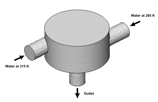
This tutorial simulates a static mixer consisting of two inlet pipes delivering water into a mixing vessel; the water exits through an outlet pipe. A general workflow is established for analyzing the flow of fluid into and out of a mixer.
Initially, water enters through both pipes at the same rate but at different temperatures. The first inlet has an initial mass flow rate of 1500 kg/s and a temperature of 315 K. The second inlet has an initial mass flow rate of 1500 kg/s and a temperature of 285 K. The radius of the mixer is 2 m.
Your goal in this tutorial is to understand how to use Design Points and DesignXplorer to maximize the amount of mixing, as measured by the range of water temperature at the outlet.
Before you begin using Ansys Workbench, you have to configure the Geometry Import option settings for use with this tutorial:
Launch Ansys Workbench.
From the Ansys Workbench menu bar, select Tools > Options.
The Options dialog box appears.
In the Options dialog box, select Geometry Import.
Ensure that Parameters is set to Independent.
Remove "DS" (and the unneeded delimiter, ";") from Filtering Prefixes and Suffixes.
Select Named Selections.
Remove "NS" from Filtering Prefixes.
Click .
To create the project, you save an empty project:
From the Ansys Workbench menu bar, select File > Save As and save the project as
StaticMixerDX.wbpjin the directory of your choice.From Toolbox > Analysis Systems, drag the Fluid Flow (CFX) system onto the Project Schematic.
Now you can create a geometry by using DesignModeler:
In the Fluid Flow (CFX) system, right-click Geometry and select New DesignModeler Geometry.
DesignModeler starts.
If DesignModeler displays a dialog box for selecting the required length unit, select Meter as the required length unit and click .
Note that this dialog box will not appear if you have previously set a default unit of measurement.
You create geometry in DesignModeler by creating two-dimensional sketches and extruding, revolving, sweeping, or lofting these to add or remove material. To create the main body of the static mixer, you will draw a sketch of a cross-section and revolve it.
In the Tree Outline, click ZXPlane.
Each sketch is created in a plane. By selecting ZXPlane before creating a sketch, you ensure that the sketch you are about to create is based on the ZX plane.
Click New Sketch
 on the Active Plane/Sketch toolbar, which is located above the
Graphics window.
on the Active Plane/Sketch toolbar, which is located above the
Graphics window. In the Tree Outline, click Sketch1.
Select the Sketching tab (below the Tree Outline) to view the available sketching toolboxes.
Before starting your sketch, set up a grid on the plane in which you will draw the sketch. The grid facilitates the precise positioning of points (when Snap is selected).
Click Settings (in the Sketching tab) to open the Settings toolbox.
Click Grid and select Show in 2D and Snap.
Click Major Grid Spacing and set it to
1.Click Minor-Steps per Major and set it to
2.To see the effect of changing Minor-Steps per Major, press and hold the right mouse button above and to the left of the plane center in the Graphics window, then drag the mouse down and right to make a box around the plane center.
When you release the mouse button, the model is magnified to show the selected area.
You now have a grid of squares with the smallest squares being 50 cm across. Because snap is selected, you can select only points that are on this grid to build your geometry. Using snap can help you to position objects correctly.
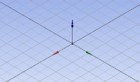
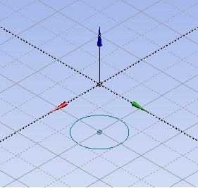
The triad at the center of the grid indicates the local coordinate frame. The color of the arrow indicates the local axis: red for X, green for Y, and blue for Z.
Start by creating the main body of the mixer:
From the Sketching tab, select the Draw toolbox.
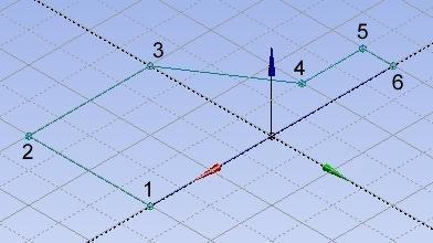
Click Polyline and then create the shape shown below as follows:
Click the grid in the position where one of the points from the shape must be placed (it does not matter which point, but a suggested order is given in the graphic below).
Click each successive point to make the shape.
If at any time you click the wrong place, right-click over the Graphics window and select Back from the shortcut menu to undo the last point selection.
To close the polyline after selecting the last point, right-click and select Closed End from the shortcut menu.
Information about the new sketch, Sketch1, appears in the details view. Note that the longest straight line (4 m long) in the diagram below is along the local X axis (located at Y = 0 m). The numbers and letters in the image below are added here for your convenience but do not appear in the software.
You will now create the main body of the mixer by revolving the new sketch around the local X axis.
Click Revolve
 from the toolbar above the Graphics window.
Details of the Revolve feature are shown in the details view at the bottom left of the window.
Leave the name of the Revolve feature at its default value:
Revolve1.Click in the details view under Details of Revolve1 > Geometry to select
Sketch1as the geometry to be revolved.The Geometry specifies which sketch is to be revolved.
In the Details View you should see Apply and Cancel buttons next to the Axis property; if those buttons are not displayed, double-click the word Axis.
In the Graphics window, click the grid line that is aligned with the local X axis (the local X axis, represented by a red arrow, is parallel to the global Z axis in this case), then click Apply in the Details View.
Leave Operation set to Add Material because you need to create a solid (which will eventually represent a fluid region).
Ensure that Angle is set to 360° and leave the other settings at their defaults.
Click Generate
 to activate the Revolve operation.
You can select this from the 3D Features Toolbar, from the shortcut menu by right-clicking in the Graphics window, or from the shortcut menu by right-clicking the Revolve1 object in the Tree Outline.
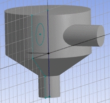
After generation, you should find that you have a solid as shown below.

To create the inlet pipes, you will create two sketches and extrude them. For clear viewing of the grid during sketching, you will hide the previously created geometry.
In the Tree Outline, click the plus sign next to 1 Part, 1 Body to expand the tree structure.
Right-click Solid and select Hide Body.
Select ZXPlane in the Tree Outline.
Click New Sketch
.From the Sketching tab, select the Draw toolbox.
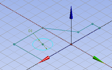
Click Circle and then create the circle shown below as follows:
Click and hold the left mouse button at the center of the circle.
While still holding the mouse button, drag the mouse to set the radius.
Release the mouse button.
Select the Dimensions toolbox, select General, click the circle in the sketch, then click near the circle to set a dimension. In the Details View, select the check box beside D1. When prompted, rename the parameter to
inDiaand click . This dimension will be a parameter that is modified in DesignXplorer.
To create the first side pipe, extrude the sketch:
Click Extrude
 from the 3D Features toolbar, located above the
Graphics window.
from the 3D Features toolbar, located above the
Graphics window.In the Details View, change Direction to Reversed to reverse the direction of the extrusion (that is, click the word Normal, then from the drop-down menu select Reversed).
Change Depth to 3 (meters) and press Enter to set this value.
All other settings should remain at their default values. Note that the Operation property is set to Add Material, which indicates that material is to be added to the existing solid.
Click Generate
to perform the extrusion.Initially, you will not see the geometry.
To see the result of the previous operation, make the solid visible:
In the Tree Outline, right-click Solid and select Show Body.
Click and hold the middle mouse button over the middle of the Graphics window and drag the mouse to rotate the model. The solid should be similar to the one shown below.
Right-click Solid and select Hide Body.
You will create the second inlet so that the relative angle between the two inlets is controlled parametrically, enabling you to evaluate the effects of different relative inlet angles:
In the Tree Outline, select ZXPlane.
In the toolbar, click New Plane
 .
.The new plane (Plane4) appears in the Tree Outline.
In the Details View, click beside Transform 1 (RMB) and choose the axis about which you want to rotate the inlet: Rotate about X.
Select the check box for the FD1, Value 1 property then, when prompted, set the name to
in2Angleand click .This makes the angle of rotation of this plane a design parameter.
Click Generate
.In the Tree Outline click Plane4.
Create a new sketch (Sketch3) based on Plane4 by clicking New Sketch
.Select the Sketching tab.
Click Settings to open the Settings toolbox.
Click Grid and select Show in 2D and Snap.
Click Major Grid Spacing and set it to 1.
Click Minor-Steps per Major and set it to 2.
Right-click over the Graphics window and select Isometric View to put the sketch into a sensible viewing position.
Zoom in, if required, to see the level of detail in the image below.
From the Draw Toolbox, select Circle and create a circle as shown below:
Select the Dimensions toolbox, click General, click the circle in the sketch, then click near the circle to set a dimension.
In the Details View, select the check box for the D1 property then, when prompted, set the name to
inDiaand click .Click Extrude
 .
.In the Details View, ensure that Direction is set to Normal in order to extrude in the same direction as the plane normal.
Ensure that Depth is set to 3 (meters).
All other settings should remain at their default values.
Click Generate
to perform the extrusion.Right-click Solid in the Tree Outline and select Show Body.
The geometry is now complete.
Named selections enable you to specify and control like-grouped items. Here, you will create named selections so that you can specify boundary conditions in CFX-Pre for these specific regions.
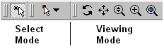
Note: The Graphics window must be in "viewing mode" for you to be able to orient the geometry, and must be in "select mode" for you to be able to select a boundary in the geometry. You set viewing mode or select mode by clicking the icons in the toolbar:
Create named selections as follows:
In viewing mode, orient the static mixer so that you can see the inlet that has the lowest value of (global) Y-coordinate.
You can rotate the mixer by holding down the middle-mouse button (or the mouse scroll wheel) while moving the mouse.
In select mode, with Selection Filter: Faces
 active (in the toolbar), click
the inlet face to select it, then right-click the inlet and select Named Selection.
active (in the toolbar), click
the inlet face to select it, then right-click the inlet and select Named Selection.In the Details View, click Apply.
Set Named Selection to
in1.Click Generate
.In viewing mode, orient the static mixer so that you can see the inlet that has the highest value of (global) Y-coordinate.
In select mode, click the inlet face to select it, then right-click the inlet and select Named Selection.
In the Details View, click Apply.
Set Named Selection to
in2.Click Generate
.In viewing mode, orient the static mixer so that you can see the outlet (the face with the lowest value of (global) Z-coordinate).
In select mode, click the outlet face to select it, then right-click the outlet and select Named Selection.
In the Details View, click Apply.
Set Named Selection to
out.Click Generate
.Click on the Ansys Workbench toolbar.
This enables you to recover the work that you have performed to this point if needed (until the next time you save the tutorial).
To create the mesh:
In the Project Schematic view, right-click the Mesh cell and select Edit.
The Meshing application appears.
Right-click Project > Model (A3) > Mesh and select .
After the mesh has been produced, return to the Project Schematic, right-click the Mesh cell, and select Update.
In the Meshing application, select File > Close Meshing.
Now that the mesh has been created, you can use CFX-Pre to define the simulation. To set up the case with CFX-Pre:
Double-click the Setup cell.
CFX-Pre appears with the mesh file loaded.
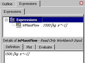
In CFX-Pre, create an expression named
inMassFlowas follows:In the Outline tree view, expand Expressions, Functions and Variables, right-click Expressions, and select Insert > Expression.
Give the new expression the name:
inMassFlowIn the Definition area, type:
1500 [kg s^-1]Click .
Right-click inMassFlow in the Expressions area and select Use as Workbench Input Parameter.
A small "P" with a right-pointing arrow appears on the expression’s icon.
Define the characteristics of the domain:
Click the Outline tab.
Double-click Simulation > Flow Analysis 1 > Default Domain to open it for editing.
Configure the following setting(s):
Tab
Setting
Value
Basic Settings
Fluid and Particle Definitions
Fluid 1
Fluid and Particle Definitions
> Fluid 1
> Material
Water
Domain Models
> Pressure
> Reference Pressure
1 [atm]
Fluids Models
Heat Transfer
> Option
Thermal Energy
Turbulence
> Option
k-Epsilon
Click OK.
Create the first inlet boundary:
From the CFX-Pre menu bar, select Insert > Boundary.
In the Insert Boundary dialog box, name the new boundary
in1and click .Configure the following setting(s) of
in1:Tab
Setting
Value
Basic Settings
Boundary Type
Inlet
Location
in1
Boundary Details
Mass and Momentum
> Option
Mass Flow Rate
Mass Flow Rate
inMassFlow [a]
Heat Transfer
> Static Temperature
315 [K]
Click OK.
Create the second inlet boundary:
From the CFX-Pre menu bar, select Insert > Boundary.
In the Insert Boundary dialog box, name the new boundary
in2and click .Configure the following setting(s) of
in2:Tab
Setting
Value
Basic Settings
Boundary Type
Inlet
Location
in2
Boundary Details
Mass and Momentum
> Option
Mass Flow Rate
Mass Flow Rate
inMassFlow [a]
Heat Transfer
> Static Temperature
285 [K]
Click OK.
Create the outlet boundary:
From the CFX-Pre menu bar, select Insert > Boundary.
In the Insert Boundary dialog box, name the new boundary
outand click .Configure the following setting(s) of
out:Tab
Setting
Value
Basic Settings
Boundary Type
Outlet
Location
out
Boundary Details
Mass and Momentum
> Option
Static Pressure
Mass and Momentum
> Relative Pressure
0 [Pa]
Click OK.
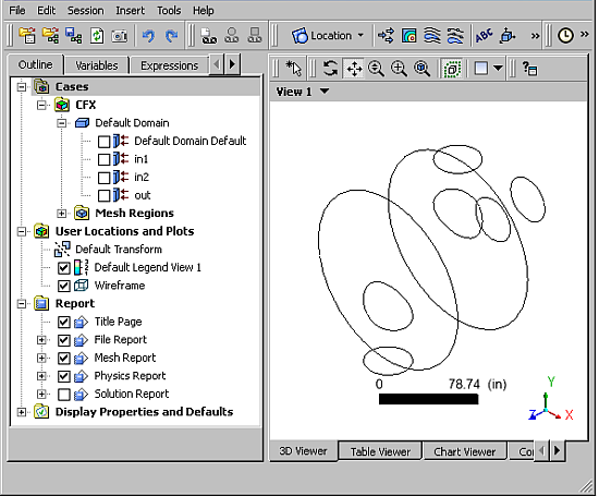
CFX-Pre and Ansys Workbench both update automatically. The three boundary conditions are displayed in the viewer as sets of arrows at the boundary surfaces. Inlet boundary arrows are directed into the domain; outlet boundary arrows are directed out of the domain.
Solver Control parameters control aspects of the numerical solution generation process. Set the solver controls as follows:
Click Solver Control
 .
.On the Basic Settings tab, set Advection Scheme > Option to
Upwind.While an upwind advection scheme is less accurate than other advection schemes, it is also more robust. This advection scheme is suitable for obtaining an initial set of results, but in general should not be used to obtain final results.
Set Convergence Control > Min. Iterations to
5.This change is required because when the solver is restarted from a previous "converged" solution for each design point, the solver may "think" the solution is converged after one or two iterations and halt the solution prematurely if the default setting (1) is maintained.
Set Convergence Control > Fluid Timescale Control > Timescale Control to
Physical Timescaleand set the physical timescale value to2[s].The time scale can be calculated automatically by the solver or set manually. The
Automaticoption tends to be conservative, leading to reliable, but often slow, convergence. It is often possible to accelerate convergence by applying a time scale factor or by choosing a manual value that is more aggressive than theAutomaticoption. By selecting a physical time scale, you obtain convergence that is at least twice as fast as with theAutomaticoption.Click .
CFX-Pre and Ansys Workbench both update automatically.
In the Project Schematic view, right-click the Solution cell and select Update.
CFX-Solver obtains a solution.
When the Solution cell shows an up-to-date state, right-click the Results cell and select Refresh.
When the refresh is complete, right-click the Results cell again and select Edit.
CFD-Post starts.

When CFD-Post starts, it displays the Outline workspace and the 3D Viewer.
You need to create an expression for the response parameter
to be examined (Outlet Temperature) called OutTempRange, which will be the maximum output temperature minus the minimum
output temperature:
On the Expressions tab, right-click in the Expressions tree view and select New.
Type
OutTempRangeand click .In the Definition area:
Right-click and select Functions > CFD-Post > maxVal.
With the cursor between the parentheses, right-click and select Variables > Temperature.
Click after the @, then right-click and select Locations > out.
Continue to edit the expression until it appears as follows:
maxVal(Temperature)@out - minVal(Temperature)@out
Click .
The new expression appears in the Expressions list. Note the value of the expression.
In the Expressions list, right-click
OutTempRangeand select Use as Workbench Output Parameter.A small "P" with a right-pointing arrow appears on the expression’s icon.
Repeat the steps above for a second expression called
OutTempAve, defined by:massFlowAve(Temperature)@out
Be sure to also set this expression to Use as Workbench Output Parameter. When you click Apply, note the value of the expression.
This expression will be used to monitor the output temperature. The overall output temperature is expected to be the average of the two input temperatures, given that the incoming mass flows are equal.
Click on the Ansys Workbench toolbar to save the project.
In CFD-Post, select File > Close CFD-Post.
Now you will manually change the values of some design parameters to see what effect each has on the rate of mixing. These combinations of parameter values where you perform calculations are called design points. As you make changes to parameters in Ansys Workbench, Ansys CFX-Pre and Ansys DesignModeler will reflect the updated values automatically. If you leave CFX-Pre and DesignModeler open, you can see the changes taking place. In particular, you can see changes in the Expressions view of CFX-Pre.
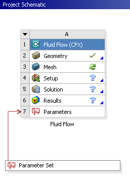
In the Project Schematic view, right-click Parameters (cell A7) and select Edit.
A Parameters tab appears.
Resize the Ansys Workbench window to be larger.
Tip: If necessary, you can close the Toolbox view to gain more space. To restore it, select View > Toolbox.
When you edit the Parameters cell (cell A7), the new views that appear on the Parameters tab are:
Outline of Schematic A7: Parameters, which lists the input and output parameters and their values (which match the values observed in previous steps).
Table of Design Points, which lists one design point named Current. Ensure that this view is wide enough to display the Retain column.
Now you will change the design parameter values from the Outline of Schematic A7: Parameters view:
On the Parameters tab, in the Outline of Schematic A7: Parameters view, change the in2Angle value from
0to-45and press Enter.Switch to the Project tab.
In the Project Schematic view, right-click Geometry and select Update.
Notice how the geometry changes in Ansys DesignModeler.
In Ansys Workbench, switch to the Parameters tab, then in the Outline of Schematic A7: Parameters view, change the in2Angle value from
-45back to0and press Enter.In the Project Schematic view, update Geometry.
Again, notice how the geometry changes in Ansys DesignModeler.
Switch to the Parameters tab, then in the Outline of Schematic A7: Parameters view, change the inMassFlow value from
1500to1600and press Enter.Notice how the value of the expression has changed in the Expressions tree view in CFX-Pre.
On the Parameters tab, in the Outline of Schematic A7: Parameters view, change the inMassFlow value from
1600back to1500and press Enter.
You have modified design parameter values and returned each to its original value. In doing this, the Outline of Schematic A7: Parameters values and the Table of Design Points values have become out-of date.
Update the current design point as follows:
Right-click any cell in the Current row of Table of Design Points and select Update Selected Design Points.
This process updates the project and all of the Ansys Workbench views. Ansys Workbench may also close any open Ansys CFX applications and run them in the background. When the update is complete, all of the results cells show current values and all of the cells that display their status are marked as being up-to-date.
Now, you will create three additional design points, DP 1, DP 2, and DP 3:
On the Parameters tab, in the Table of Design Points view in the line under Current, make the following entries to create design point DP 1:
P1 - inDia:
1P2 - in2Angle:
-45P3 - inMassFlow:
1500Retain:
(Selected)
Note: You should save the project once before you retain a design point.
Right-click in the row for DP 1 and select Update Selected Design Points.
Ansys Workbench recalculates all of the values for the input and output parameters. All of the views are updated.
Create design point DP 2 using these values:
P1 - inDia:
1.5P2 - in2Angle:
0P3 - inMassFlow:
1500Retain:
(Selected)
Right-click in the row for DP 2 and select Update Selected Design Points.
Create design point DP 3 using these values:
P1 - inDia:
1P2 - in2Angle:
0P3 - inMassFlow:
1600Retain:
(Selected)
In the Ansys Workbench toolbar, click Update All Design Points.
This command updates any out-of-date design points in a sequential fashion.
On the Ansys Workbench toolbar, click to save the project.
Recall that the goal of this design study is to maximize the
amount of mixing by finding the minimum value of OutTempRange.
Note that OutTempRange varies significantly due to changes in the input parameters.
Also note that, as expected, OutTempAve stays very near 300 K.
In the next section you will automate the process of changing input parameters by using Design Exploration.
In this section you will use Design Exploration's Response Surface Optimization feature to minimize the value of
OutTempRange.
Return to the Project tab.
If you need to restore the Toolbox, select View > Toolbox. If no systems appear in the Toolbox, select a cell in the Project Schematic view to refresh Ansys Workbench.
From the Design Exploration toolbox, drag a Response Surface Optimization system to the Project Schematic (under the Parameter Set bar).
Edit the Design of Experiments cell.
On the B2:Design of Experiments tab, in the Outline of Schematic B2: Design of Experiments view:
Select the Enabled check boxes next to P2 - in2Angle (cell A6) and P3 - inMassFlow (cell A7), and clear the check box next to P1 - inDia (cell A5).
Select cell P3 - inMassFlow (cell A7) then, in the Properties of Outline A7: P3 - inMassFlow view, set:
Lower Bound: 1000
Upper Bound: 2000
Select cell P2 - in2Angle (cell A6) then, in the Properties of Outline A6: P2 - in2Angle view, set:
Lower Bound: -45
Upper Bound: 0
In the Ansys Workbench menu bar, ensure that View > Table is selected.
On the B2:Design of Experiments tab, on the toolbar, click .
The table of design points has nine entries in the Name column, each of which represents a solver run to be performed. Beside the Name column are columns that have the values for the two input parameters, and a column to hold the value the solver will obtain for the output parameter.
In the Project Schematic view, update the Design of Experiments cell. You can monitor the progress of the solver runs by clicking in the lower-right corner of the Ansys Workbench window.
When the processing is complete, the table of design points (on the B2:Design of Experiments tab) displays the results. Click the down-arrow on the P4 - OutTempRange (K) cell to sort the design points according to the value of
OutTempRange. Note that, in this case and for the range of inputs considered, the best results are returned from the lowest mass flow rate and an input angle of zero.
To view the response surface for this experiment:
In the Ansys Workbench menu bar, ensure that View > Chart is selected.
In the Project Schematic view, update the Response Surface.
Right-click Response Surface and select Edit to open the B3:Response Surface tab.
In the Outline of Schematic B3: Response Surface view, select Response Surface > Response Points > Response Point > Response. The results appear in various views:
The Toolbox shows the types of charts that are available.
If the Toolbox is not visible, you can show it by selecting View > Toolbox.
Response Chart for P4 - OutTempRange shows a 2D graph comparing
OutTempRangetoin2Angle.The Properties of Outline A20: Response shows the values that are being used to display the 2D graph. Note that the other variable that was considered in the Design of Experiments,
inMassFlow, is held at1500.
In the Properties of Outline A20: Response view, select Chart > Mode > 3D. A 3D chart appears, showing the full range of inMassFlow results. The chart shows that, in this case and for the range of inputs considered, the best results are returned from the lowest mass flow rate and an input angle of zero.
To view the optimization for this experiment:
In the Project Schematic view, edit the Optimization cell.
On the B4:Optimization tab, in the Outline of Schematic B4: Optimization view, select Objectives and Constraints.
In the Table of Schematic B4: Optimization view, add the following objective:
Parameter:
P4 - OutTempRangeType:
Minimize
The Objective Name is automatically set to
Minimize P4.In the Project Schematic view, right-click Optimization and select Update.
On the B4:Optimization tab, in Outline of Schematic B4: Optimization, select Optimization > Results > Candidate Points.
In the Table of Schematic B4: Optimization, Candidate Points view, three design point candidates appear with their interpolated values.
Recall that design points are combinations of parameter values where you perform real calculations (rather than relying on the interpolated values that appear in the response charts). All of the candidates are represented graphically in the Candidate Points chart.
In Table of Schematic B4: Optimization, Candidate Points, right-click Candidate Point 1 and select Insert as Design Point.
Switch to the Parameters tab.
The various views update and a new design point has appeared in Table of Design Points.
In Table of Design Points, the new design point, DP 4 has no values and requests an update. Right-click the lightning icon and select Update Selected Design Points.
You can follow the progress of the update in the Project Schematic view while Ansys Workbench reruns its calculations for the design point parameters.
Note that the resulting value of
OutTempRangefor DP 4 in Table of Design Points is the result of a solver calculation, and differs slightly from the value ofOutTempRangeinterpolated from the response surface for Candidate Point 1.