


This tutorial includes:
In this tutorial you will learn about:
Preparing and running a series of related simulations to generate cavitation performance data for a pump.
Creating a drop curve chart in CFD-Post.
Using isosurfaces in CFD-Post to visualize regions of cavitation.
Component | Feature | Details |
|---|---|---|
CFX-Pre | User Mode | General mode |
Analysis Type | Steady State | |
Fluid Type | Water at 25 C | |
Water Vapour at 25 C | ||
Fluid Models | Homogeneous Model | |
Domain Type | Single Domain | |
Turbulence Model | k-Epsilon | |
Heat Transfer | Isothermal | |
Boundary Conditions | Inlet (Subsonic) | |
Outlet (Subsonic) | ||
Wall (Counter Rotating) | ||
| Timestep | Physical Time Scale | |
| CFD-Post | Plots | Contour |
This tutorial uses a simple pump to illustrate the basic concepts of setting up, running, and postprocessing a cavitation problem in Ansys CFX.
When liquid is suddenly accelerated in order to move around an obstruction, a decrease in the local pressure is present. Sometimes, this pressure decrease is substantial enough that the pressure falls below the saturation pressure determined by the temperature of the liquid. In such cases, the fluid begins to vaporize in a process called cavitation. Cavitation involves a very rapid increase in the volume occupied by a given mass of fluid, and when significant, can influence the flow distribution and operating performance of the device. In addition, the vaporization of the liquid, and the subsequent collapse of the vapor bubbles as the local pressure recovers, can cause damage to solid surfaces. For these reasons (among others), it is desirable, in the design and operation of devices required to move liquid, to be able to determine if cavitation is present, including where and the extent of the cavitation. Furthermore it is also useful to examine this behavior for a range of conditions.
The model conditions for this example are turbulent and incompressible. The speed and direction of rotation of the pump is 132 rad/sec about the Z axis (positive rotation following the right hand rule). The relevant problem parameters are:
Inflow total pressure = 100000 Pa
Outflow mass flow = 16 kg/s
Inlet turbulence intensity = 0.03
Inlet length scale = 0.03 m
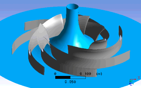
The SHF (Societe Hydraulique Francaise) pump has seven impeller blades. Due to the periodic nature of the geometry, only a single blade passage of the original pump must be modeled, therefore minimizing the computer resources required to obtain a solution.
The objective of this tutorial is to show pump cavitation performance in the form of a drop curve. The drop curve is a chart of Head versus Net Positive Suction Head (NPSH). This tutorial provides the data for the drop curve, but also has instructions for optionally generating the data by running a series of simulations with progressively lower inlet pressures. Each simulation is initialized with the results of the previous simulation.
If this is the first tutorial you are working with, it is important to review the following topics before beginning:
Create a working directory.
Ansys CFX uses a working directory as the default location for loading and saving files for a particular session or project.
Download the
drop_curve.zipfile here .Unzip
drop_curve.zipto your working directory.Ensure that the following tutorial input file is in your working directory:
Cavitation.gtm
Set the working directory and start CFX-Pre.
For details, see Setting the Working Directory and Starting Ansys CFX in Stand-alone Mode.
A steady-state high-pressure (inlet pressure of 100,000 Pa) simulation of the pump without cavitation (that is, simulation of the pump without water vapor) will first be set up and run to provide initial values for a cavitation simulation later on in the tutorial.
In CFX-Pre, select File > New Case.
Select General and click .
Select File > Save Case As.
Under File name, type CavitationIni.
Click .
Right-click
Meshand select Import Mesh > CFX Mesh.The Import Mesh dialog box appears.
Configure the following setting(s):
Setting
Value
File name
Cavitation.gtm
Click Open.
Because this tutorial uses water at 25 °C and water vapor at 25 °C, you need to load these materials. Note that you will use only the liquid water for the first part of the tutorial. The vapor is being loaded now in anticipation of using it for the cavitation model later in the tutorial.
In the Outline tree view, right-click
Simulation>Materialsand select Import Library Data.The Select Library Data to Import dialog box is displayed.
Expand
Water Data.While holding down the Ctrl key, select both
Water Vapour at 25 CandWater at 25 C.Click .
Edit
Case Options>Generalin the Outline tree view and ensure that Automatic Default Domain is turned on.A domain named
Default Domainshould appear under theSimulationbranch.Rename
Default DomaintoPump.Edit
Pump.Under Fluid and Particle Definitions, delete
Fluid 1and create a new fluid definition namedLiquid Water.Configure the following setting(s):
Tab
Setting
Value
Basic Settings
Fluid and Particle Definitions
Liquid Water
Fluid and Particle Definitions
> Liquid Water
> Material
Water at 25 C [a]
Domain Models
> Pressure
> Reference Pressure
0 [atm]
Domain Models
> Domain Motion
> Option
Rotating
Domain Models
> Domain Motion
> Angular Velocity
132 [radian s^-1]
Fluid Models
Turbulence
> Option
k-Epsilon
Click .
Create a new boundary named
Inlet.Configure the following setting(s):
Tab
Setting
Value
Basic Settings
Boundary Type
Inlet
Location
INBlock INFLOW
Boundary Details
Mass And Momentum
> Option
Stat. Frame Tot. Press.
Mass And Momentum
> Relative Pressure
100000 [Pa]
Flow Direction
> Option
Cartesian Components
Flow Direction
> X Component
0
Flow Direction
> Y Component
0
Flow Direction
> Z Component
1
Turbulence
> Option
Intensity and Length Scale
Turbulence
> Option
> Fractional Intensity
0.03
Turbulence
> Option
> Eddy Length Scale
0.03 [m]
Click .
Create a new boundary named
Outlet.Configure the following setting(s):
Tab
Setting
Value
Basic Settings
Boundary Type
Outlet
Location
OUTBlock OUTFLOW
Boundary Details
Mass and Momentum
> Option
Mass Flow Rate
Mass and Momentum
> Mass Flow Rate
16 [kg/s]
Click .
Set up the hub and shroud to be a stationary (non-rotating) wall.
Create a new boundary named
Stationary Wall.Configure the following setting(s) of
Stationary Wall:Tab
Setting
Value
Basic Settings
Boundary Type
Wall
Location
OUTBlock HUB, OUTBlock SHROUD [a]
Boundary Details
Mass and Momentum
> Wall Velocity
(Selected)
Mass and Momentum
> Wall Velocity
> Option
Counter Rotating Wall
Click .
Click Insert > Domain Interface and, in the dialog box that appears, set Name to
Periodic Interfaceand click .Configure the following setting(s) of
Periodic Interface:Tab
Setting
Value
Basic Settings
Interface Side 1
> Region List
INBlock PER1, OUTBlock PER1, Passage PER1
Interface Side 2
> Region List
INBlock PER2, OUTBlock PER2, Passage PER2
Interface Models
> Option
Rotational Periodicity
Click .
Select Insert > Domain Interface and in the dialog box that appears, set Name to
Inblock to Passage Interfaceand click .Configure the following settings of
Inblock to Passage Interface:Tab
Setting
Value
Basic Settings
Interface Side 1
> Region List
OUTFLOW INBlock
Interface Side 2
> Region List
INFLOW Passage
Mesh Connection
Mesh Connection Method
> Mesh Connection
> Option
1:1
Click .
Select Insert > Domain Interface and in the dialog box that appears, set the Name to
Passage to Outblock Interfaceand click .Configure the following settings of
Passage to Outblock Interface:Tab
Setting
Value
Basic Settings
Interface Side 1
> Region List
OUTFLOW Passage
Interface Side 2
> Region List
INFLOW OUTBlock
Mesh Connection
Mesh Connection Method
> Mesh Connection
> Option
1:1
Click .
With the boundary conditions and domain interfaces defined above, the default boundary of a rotating wall is applied to the blade and the upstream portions of the hub and shroud.
The initial values that will be set up are consistent with the inlet boundary conditions settings.
Click Global Initialization
 .
.Configure the following setting(s):
Tab
Setting
Value
Global Settings
Initial Conditions
> Cartesian Velocity Components
> Option
Automatic with Value
Initial Conditions
> Cartesian Velocity Components
> U
0 [m/s]
Initial Conditions
> Cartesian Velocity Components
> V
0 [m/s]
Initial Conditions
> Cartesian Velocity Components
> W
1 [m/s]
Initial Conditions
> Static Pressure
> Option
Automatic with Value
Initial Conditions
> Static Pressure
> Relative Pressure
100000 [Pa]
Initial Conditions
> Turbulence
> Option
Intensity and Length Scale
Initial Conditions
> Turbulence
> Fractional Intensity
> Option
Automatic with Value
Initial Conditions
> Turbulence
> Fractional Intensity
> Value
0.03
Initial Conditions
> Turbulence
> Eddy Length Scale
> Option
Automatic with Value
Initial Conditions
> Turbulence
> Eddy Length Scale
> Value
0.03 [m]
Click .
Click Solver Control
 .
.Configure the following setting(s):
Tab
Setting
Value
Basic Settings
Convergence Control
> Max Iterations
500
Convergence Control
> Fluid Timescale Control
> Timescale Control
Physical Timescale
Convergence Control
> Fluid Timescale Control
> Physical Timescale
1e-3[s] [a]
Convergence Criteria
> Residual Target
7.5e-6
Click .

CFX-Solver Manager should be running. You will be able to obtain a solution to the CFD problem by following the instructions below.
Ensure that the Define Run dialog box is displayed.
Click .
You may see a notice about an artificial wall at the inlet. This notice indicates that the flow is trying to exit at the inlet. This can be ignored because the amount of reverse flow is very low.
CFX-Solver runs and attempts to obtain a solution. At the end of the run, a dialog box is displayed stating that the simulation has ended.
Select Post-Process Results.
If using stand-alone mode, select Shut down CFX-Solver Manager.
Click OK.
CFD-Post should be running.
This case is run with temperatures around 300 K. The vapor pressure of water at this temperature is around 3574 Pa. To confirm that water vapor or cavitation is not likely for this operating condition of the pump, an isosurface of pressure at 3574 Pa will be created.
Create an isosurface of pressure at 3574 [Pa]:
Select Insert > Location > Isosurface and accept the default name.
Configure the following setting(s) in the details view:
Tab
Setting
Value
Geometry
Definition
> Variable
Pressure
Definition
> Value
3574 [Pa]
Click .
Notice that the isosurface does not appear. There is no place in the blade passage where the pressure is equal to 3574 Pa, which implies that there is no water vapor.
Quit CFD-Post, saving the state at your discretion.
The simulation will be modified in CFX-Pre to include water vapor and enable the cavitation model. Monitor points will also be defined to observe the Net Positive Suction Head (NSPH) and pressure head values.
The following topics are discussed:
Ensure that the following tutorial input files are in your working directory:
CavitationIni.cfx
CavitationIni_001.res
Set the working directory and start CFX-Pre if it is not already running.
For details, see Setting the Working Directory and Starting Ansys CFX in Stand-alone Mode.
Open CavitationIni.cfx and save it as Cavitation_100000.cfx.
"100000" indicates the inlet pressure of the simulation.
Open
Pumpfor editing.In the Fluid and Particle Definitions section, click Add new item
 and name it
 Water Vapor.Configure the following setting(s):
Tab
Setting
Value
Basic Settings
Fluid and Particle Definitions
Liquid Water
Fluid and Particle Definitions
> Liquid Water
> Material
Water at 25 C [a]
Fluid and Particle Definitions
Water Vapor
Fluid and Particle Definitions
> Water Vapor
> Material
Water Vapour at 25 C
Fluid Models
Multiphase
> Homogeneous Model
(Selected) [b]
Fluid Pair Models
Fluid Pair
> Liquid Water | Water Vapor
> Mass Transfer
> Option
Cavitation
Fluid Pair
> Liquid Water | Water Vapor
> Mass Transfer
> Cavitation
> Option
Rayleigh Plesset
Fluid Pair
> Liquid Water | Water Vapor
> Mass Transfer
> Cavitation
> Mean Diameter
2e-6 [m]
Fluid Pair
> Liquid Water | Water Vapor
> Mass Transfer
> Cavitation
> Saturation Pressure
(Selected)
Fluid Pair
> Liquid Water | Water Vapor
> Mass Transfer
> Cavitation
> Saturation Pressure
> Saturation Pressure
3574 [Pa] [c]
Click the Ellipsis icon
 to open the Material dialog box, then click
the Import Library Data icon to open the Select Library Data to Import dialog box. In that dialog
box, expand
to open the Material dialog box, then click
the Import Library Data icon to open the Select Library Data to Import dialog box. In that dialog
box, expand Water Datain the tree, then selectWater at 25 Cand click .The homogeneous model will be selected because the interphase transfer rate is very large in the pump. This results in all fluids sharing a common flow field and turbulence.
The pressure for a corresponding saturation temperature at which the water in the pump will boil into its vapor phase is 3574 Pa.
Click .
Error messages appear, but you will correct those problems in the next steps.
Open
Inletfor editing and configure the following setting(s):Note that you are setting the inlet to have 100% liquid water. Consequently, at the inlet, the volume fraction of liquid water is 1 and the volume fraction of vapor is 0.
Tab
Setting
Value
Fluid Values
Boundary Conditions
Liquid Water
Boundary Conditions
> Liquid Water
> Volume Fraction
> Volume Fraction
1
Boundary Conditions
Water Vapor
Boundary Conditions
> Water Vapor
> Volume Fraction
> Volume Fraction
0
Click .
Open
Outletfor editing.On the Boundary Details tab, set Mass and Momentum > Option to
Bulk Mass Flow
Rate
and Mass Flow Rate to16 [kg s^-1].Click .
The problems have been resolved and the error messages have disappeared.
Expressions defining the Net Positive Suction Head (NPSH) and Head are created in order to monitor their values as the inlet pressure is decreased. By monitoring these values, a drop curve can be produced.
Create the following expressions.
Name | Definition |
|---|---|
Ptin | massFlowAve(Total Pressure in Stn Frame)@Inlet |
Ptout | massFlowAve(Total Pressure in Stn Frame)@Outlet |
Wden | 996.82 [kg m^-3] |
Head | (Ptout-Ptin)/(Wden*g) |
NPSH | (Ptin- Pvap)/(Wden*g) |
Pvap | 3574 [Pa] |
Two monitor points will be added to track the NPSH and head using the expressions created in the previous step.
Click Output Control
 .
.On the Monitor tab, select Monitor Objects and click Add new item
.Enter
NPSH Pointas the name of the monitor point, then configure the following settings:Tab
Setting
Value
Monitor
Monitor Objects
> Monitor Points and Expressions
> NPSH Point
> Option
Expression
Monitor Objects
> Monitor Points and Expressions
> NPSH Point
> Expression Value
NPSH
Create a second monitor point named
Head Pointwith the same parameters as the first, with the exception that Expression Value is set toHead.Click .
CFX-Solver Manager should be running. Obtain a solution to the CFD problem by following these instructions:
Ensure that the Define Run dialog box is displayed.
Under the Initial Values tab, select Initial Values Specification.
Select CavitationIni_001.res for the initial values file using the Browse
 tool.
tool.Click Start Run.
You may see a notice about an artificial wall at the inlet. This notice indicates that the flow is trying to exit at the inlet. This can be ignored because the amount of reverse flow is very low.
CFX-Solver runs and attempts to obtain a solution. A dialog box is displayed stating that the simulation has ended.
Select Post-Process Results.
If using stand-alone mode, select Shut down CFX-Solver Manager.
Click OK.
You will create an isosurface to observe the volume fraction of water vapor at 25 °C. Note that the pressure below the threshold is the same as found earlier in Simulating the Pump with High Inlet Pressure.
Create an isosurface for the volume fraction of water vapor at 25 °C, at 0.1:
CFD-Post should be running; start it if necessary.
Click Insert > Location > Isosurface and accept the default name.
Configure the following setting(s) in the details view:
Tab
Setting
Value
Geometry
Definition
> Variable
Water Vapor.Volume Fraction
Definition
> Value
0.1
Click .
Notice that the isosurface is clear. There is no water vapor at 25 °C in the blade passage for the simulation with cavitation because at an inlet total pressure of 100000 Pa, the minimum static pressure in the model is above the vapor pressure.
Quit CFD-Post saving the state at your discretion.
In order to construct a drop curve for this cavitation case, the inlet pressure must be decremented from its initial value of 100000 Pa to 17500 Pa, and the Head and NPSH values must be recorded for each simulation. The results are provided in Table 26.1: Pump Performance Data.
Table 26.1: Pump Performance Data
Inlet Pressure Pa | NPSH m | Head m |
|---|---|---|
100000 | 9.859e+00 | 3.537e+01 |
80000 | 7.813e+00 | 3.535e+01 |
60000 | 5.767e+00 | 3.535e+01 |
40000 | 3.721e+00 | 3.536e+01 |
30000 | 2.698e+00 | 3.538e+01 |
20000 | 1.675e+00 | 3.534e+01 |
18000 | 1.470e+00 | 3.528e+01 |
17500 | 1.419e+00 | 3.184e+01 |
Optionally, if you want to generate the data shown in Table 26.1: Pump Performance Data, then follow the instructions in the following two sections (Writing CFX-Solver Input (.def) Files for Lower Inlet Pressures and Obtaining the Solutions using CFX-Solver Manager). Those instructions involve running several simulations in order to obtain a set of results files. As a benefit to doing this, you will have the results files required to complete an optional postprocessing exercise at the end of this tutorial. This optional postprocessing exercise involves using isosurfaces to visualize the regions of cavitation, and visually comparing these isosurfaces between different results files.
If you want to use the provided table data to produce a drop curve, proceed to Generating a Drop Curve.
Produce a set of definition (.def)
files for the simulation, with each definition file specifying a progressively
lower value for the inlet pressure:
CFX-Pre should be running; start it if necessary.
Open
Cavitation_100000.cfx.Open
Simulation>Flow Analysis 1>Pump>Inlet.On the Boundary Details tab change Mass and Momentum > Relative Pressure to
80000 [Pa].Click .
Right-click
Simulationand select Write Solver Input File.Set File name to
Cavitation_80000.def.Click .
Change the inlet pressure and save a corresponding CFX-Solver input file for each of the 6 other pressures: 60000 Pa, 40000 Pa, 30000 Pa, 20000 Pa, 18000 Pa, and 17500 Pa.
Note: There are other techniques for defining a set of related simulations. For example, you could use configuration control, as demonstrated in Flow from a Circular Vent.
Run each of the CFX-Solver input files that you created in the previous step:
Start CFX-Solver Manager if it is not already running.
Ensure that the Define Run dialog box is displayed.
Under Solver Input File, click Browse
and select Cavitation_80000.def.Under the Initial Values tab, select Initial Values Specification.
Select
Cavitation_100000_001.resfor the initial values file using the Browse tool.Click Start Run.
You may see a notice about an artificial wall at the inlet. This notice indicates that the flow is trying to exit at the inlet. This can be ignored because the amount of reverse flow is very low.
CFX-Solver runs and attempts to obtain a solution. At the end of the run, a dialog box is displayed stating that the simulation has ended.
Clear Post-Process Results.
Click .
Repeat this process until you have run all the CFX-Solver input files for all 6 other inlet pressures: 60000 Pa, 40000 Pa, 30000 Pa, 20000 Pa, 18000 Pa, and 17500 Pa.
Note that each solver run should be initialized using the previous run's results (
.res) file.
The pump simulation with cavitation and an inlet pressure of 17500 Pa converges rather poorly. The converge failure indicates that the numerical results are unreliable. However, for a pump designed to avoid significant cavitation while operating, you can use the solutions that do converge well to help establish the operating range and pump performance within that range.
To see the pump performance, you will generate a drop curve to show the pump performance over a range of inlet pressures. After generating the drop curve, there is an optional exercise for visualizing the cavitation regions using isosurfaces.
The optional exercise of visualizing the cavitation regions requires the results files from the 60000 Pa, 40000 Pa, 20000 Pa, and 17500 Pa simulations. If you have not generated those results files and want to complete the optional exercise, then generate the results files by following the instructions in:
To generate a drop curve, you will need the values for Net Positive Suction Head (NPSH) and head as the inlet pressure decreases. This data is provided in Table 26.1: Pump Performance Data. If you want to use that data, proceed to Creating a Table of the Head and NPSH Values. If you have chosen to run all of the simulations and have obtained all of the results files, you can obtain the drop curve data yourself by following the instructions in the Creating a Head-versus-NPSH Chart (Optional Exercise) section.
Start CFD-Post.
Click Insert > Table and set the name to
Drop Curve Values.Enter the values from Table 26.1: Pump Performance Data for the 8 inlet pressures in the table.
Enter the NPSH values in the left column and the head values in the right column.
Click Save Table
 , and configure the following setting(s):
Setting
Value
File name
Drop Curve Values
Files of type
Comma Separated Values — Excel Readable (*.csv)
Click Save.
Click Insert > Chart.
Set the name to
Drop Curveand click OK.Configure the following setting(s):
Tab
Setting
Value
General
Title
Drop Curve
Data Series
Data Source
> File
(Selected)
Data Source
> File
> Browse
Drop Curve Values.csv [a]
X Axis
Axis Range
> Determine ranges automatically
(Cleared)
Axis Range
> Min
0
Axis Range
> Max
10
Axis Labels
> Use data for axis labels
(Cleared)
Axis Labels
> Custom Label
NPSH [m]
Y Axis
Axis Range
> Determine ranges automatically
(Cleared)
Axis Range
> Min
0
Axis Range
> Max
45
Axis Labels
> Use data for axis labels
(Cleared)
Axis Labels
> Custom Label
Head [m]
Line Display
Line Display
> Symbols
Triangle
Click .
Here is what the drop curve created in the earlier steps should look like:
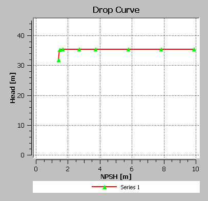
You can see here that there is not significant degradation in the performance curve as the inlet total pressure is dropped. This is due to the fact that, for a part of the test, the inlet total pressure is sufficiently high to prevent cavitation, which implies that the normalized pressure rise across the pump is constant. Also, although you may start at a high inlet pressure where there is no cavitation, as you drop the inlet pressure, cavitation will appear but will have no significant impact on performance (incipient cavitation) until the blade passage has sufficient blockage due to vapor. At that point, performance degrades.
When the inlet total pressure reaches a sufficiently low value, cavitation occurs. What is called the point of cavitation is often marked by the NPSH value at which the pressure rise has fallen by a few percent. In this tutorial, although the drop curve does appear to drop by at least a few percent, the shape of the curve is unreliable for inlet total pressures at or below 18000 Pa due to convergence failure. Therefore in this tutorial, the point of cavitation is not known with accuracy, but could be considered to be near or below the NPSH value at which the inlet total pressure is 20000 Pa.
Important: If you want to complete an optional exercise on visualizing the cavitation regions, proceed to Visualizing the Cavitation Regions (Optional Exercise). Otherwise, quit CFD-Post, saving the state at your discretion.
Start CFD-Post.
To load the results file, select File > Load Results or click Load Results
 .
.On the right side of the Load Results File dialog box, note down the current setting under CFX run history and multi-configuration options. Set this option to Load complete history as: > A single case, unless already set.
Important: This setting, under CFX run history and multi-configuration options, persists when you close CFD-Post. Ensure that you set this back to the original setting noted above, as instructed to do so at the end of the tutorial. Not doing so could lead to undesirable results when postprocessing other cases.
In the Load Results File dialog box, select
Cavitation_17500_001.res.Click Open.
When you started the CFX-Solver run using initial values, by default the Continue History From option was on. This enables the results file to retain a reference to the initial value results file. When the final results file is loaded into CFD-Post using the Load complete history as: A single case, it includes results from all the initial values files as well as the final results. Each of the previous initial values files is available as a time step (in this case a sequence) through the Timestep Selector.
Click when prompted with a Process Multiple Results as a Sequence message.
Click Insert > Chart or click Chart
 .
.Set the name to
Drop Curveand click OK.Configure the following setting(s):
Tab
Setting
Value
General
Type
XY - Transient or Sequence
Title
Drop Curve
Data Series
Data Source
> Expression
(Selected)
Data Source
> Expression
Head
X Axis
Data Selection
> Expression
NPSH
Y Axis
Axis Range
> Determine ranges automatically
(Cleared)
Axis Range
> Min
0
Axis Range
> Max
45
Line Display
Line Display
> Symbols
Triangle
Click .
Here is what the drop curve created in the earlier steps should look like:
You can see here that there is not significant degradation in the performance curve as the inlet total pressure is dropped. This is due to the fact that, for a part of the test, the inlet total pressure is sufficiently high to prevent cavitation, which implies that the normalized pressure rise across the pump is constant. Also, although you may start at a high inlet pressure where there is no cavitation, as you drop the inlet pressure, cavitation will appear but will have no significant impact on performance (incipient cavitation) until the blade passage has sufficient blockage due to vapor. At that point, performance degrades.
When the inlet total pressure reaches a sufficiently low value, cavitation occurs. What is called the point of cavitation is often marked by the NPSH value at which the pressure rise has fallen by a few percent. In this tutorial, although the drop curve does appear to drop by at least a few percent, the shape of the curve is unreliable for inlet total pressures at or below 18000 Pa due to convergence failure. Therefore in this tutorial, the point of cavitation is not known with accuracy, but could be considered to be near or below the NPSH value at which the inlet total pressure is 20000 Pa.
Important: If you want to complete an optional exercise on visualizing the cavitation regions, proceed to Visualizing the Cavitation Regions (Optional Exercise). Otherwise, proceed to Restoring CFX run history and multi-configuration options.
This is an optional part of the tutorial that requires the results files from the 60000 Pa, 40000 Pa, 20000 Pa, and 17500 Pa simulations. If you have not generated those results files and want to complete this optional exercise, then generate the results files by following the instructions in:
Cavitation does not occur for the 100000 Pa and 80000 Pa simulations. Create an isosurface for 10% water vapor (by volume fraction), for the 60000 Pa, 40000 Pa, 20000 Pa, and 17500 Pa simulations:
Use
Cavitation_60000_001.resto create an isosurface:Launch CFD-Post and load
Cavitation_60000_001.res.Select Insert > Location > Isosurface and accept the default name.
Configure the following setting(s) in the details view:
Tab
Setting
Value
Geometry
Definition
> Variable
Water Vapor.Volume Fraction
Definition
> Value
0.1
Click .
Add
Cavitation_40000_001.resto the current results:Select File > Load Results.
Under Case options, select both Keep current cases loaded and Open in new view.
Select
Cavitation_40000_001.res.Click Open.
Click a blank area inside the viewport named View 2 (which contains the results that you just loaded) to make that viewport active, then turn on visibility for the isosurface in the Outline tree view.
In a similar way, load
Cavitation_20000_001.resandCavitation_17500_001.resand make the isosurface visible on these results.Click Synchronize camera in displayed views
 so that all viewports maintain the same camera
position.
so that all viewports maintain the same camera
position.Rotate the view (from any viewport) to inspect the results.
Observe that the amount of water vapor increases as the inlet pressure decreases.
Important: If you created the drop curve by setting the CFX run history and multi-configuration options, proceed to Restoring CFX run history and multi-configuration options. Otherwise, quit CFD-Post, saving the state at your discretion.
As mentioned above the setting under CFX run history and multi-configuration options persists when you close CFD-Post. This section outlines the steps to restore CFX run history and multi-configuration options to its original setting.
Select File > Close to close the current file.
Click Close if prompted to save.
Load a results file by selecting File > Load Results or click Load Results
.On the right side of the Load Results File dialog box, restore the original settings under CFX run history and multi-configuration options.
In the Load Results File dialog box, select
Cavitation_17500_001.res.Click Open.
Quit CFD-Post, by selecting File > Quit.