


This tutorial includes:
In this tutorial you will learn about:
Importing a CCL file in CFX-Pre.
Editing and creating boundary conditions in CFX-Pre.
Adding particles that evaporate.
Creating a domain interface in CFX-Pre.
Creating contour plots and inserting particle tracking in CFD-Post.
Component | Feature | Details |
|---|---|---|
CFX-Pre
| User Mode | General mode |
Analysis Type | Steady State | |
Fluid Type | General Fluid | |
Domain Type | Single Domain | |
Boundary Conditions | Water Nozzle | |
Air Inlet | ||
Outlet | ||
Domain 1 Default | ||
Domain Interface | Fluid Fluid | |
Timescale | Physical Timescale | |
Particle Coupling Control | Selected | |
Extra Output Variables List | Selected | |
CFD-Post | Plots | Contour Plots |
Particle Tracking |
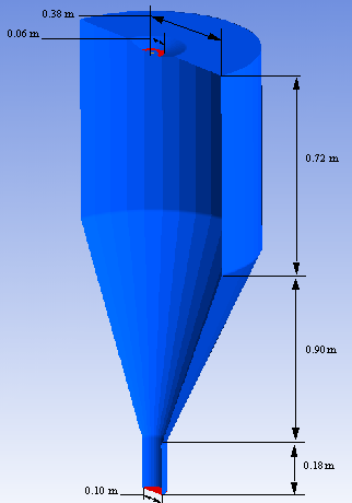
In this example, a spray dryer is modeled in which water drops are evaporated by a hot air flow. The goal of this tutorial is to observe the variation of gas temperature and mass fraction of water vapor, and of averaged values of mean droplet diameter and droplet temperature in the spray dryer, as well as the temperature and size of individual water drops as they travel through the spray dryer.
The following figure shows approximately half of the full geometry.
The spray dryer has two inlets named Water Nozzle and Air Inlet, and one outlet named Outlet. The Water Nozzle is where
the liquid water enters in a primary air flow at a mass flow rate
of 1.33e-4 kg/s. The Air Inlet is for the swirling,
drying air flow. The Water Nozzle inlet is located
in the middle of the circular Air Inlet. When
the spray dryer is operating, the inlets are located at the top of
the vessel and the outlet at the bottom.
Periodic boundaries are used to enable only a small section of the full geometry to be modeled. The geometry to be modeled consists of a 9 degree section of the axisymmetric dryer shape. The relevant parameters of this problem are:
Static temperature at
Water Nozzle= 300 KSize distribution for the drops being created by the
Water Nozzleis prescribed using discrete diameter values and associated fractions of the droplet mass flow rate.Air Inletmass and momentum axial component = 30 m/s (downwards along the axis of the spray dryer),Air Inletmass and momentum radial component = 0 m/s,Air Inletmass and momentum theta component = 10 m/sStatic temperature at
Air Inlet= 423 KRelative pressure at
Outlet= 0 PaNormal speed of Water = 10 m/s
The approach for solving this problem is to first import a CCL file with the fluid properties, domain and boundary conditions in CFX-Pre. Minor changes will be made to the information imported from the CCL file. Boundary conditions and a domain interface will also be added. In CFD-Post, contour plots will be created to see the variation of temperature, mass fraction of water, average mean particle diameter of liquid water, and averaged temperature of liquid water in the spray dryer. Finally, particle tracking will be used for plotting the temperature of liquid water.
If this is the first tutorial you are working with, it is important to review the following topics before beginning:
Create a working directory.
Ansys CFX uses a working directory as the default location for loading and saving files for a particular session or project.
Download the
spray_dryer.zipfile hereUnzip
spray_dryer.zipto your working directory.Ensure that the following tutorial input file is in your working directory:
spraydryer9.gtm
Set the working directory and start CFX-Pre.
For details, see Setting the Working Directory and Starting Ansys CFX in Stand-alone Mode.
This section describes the step-by-step definition of the flow physics in CFX-Pre for a steady-state simulation.
In CFX-Pre, select File > New Case.
Select General and click .
Edit
Case Options>Generalin the Outline tree view and ensure that Automatic Default Domain is turned off.Click .
Select File > Save Case As.
Under File name, type
SprayDryer.Click .
Later in this tutorial, you will import a template that sets up, among other things, a domain.
Right-click
Meshand select Import Mesh > CFX Mesh.The Import Mesh dialog box appears.
Configure the following setting(s):
Setting
Value
File name
spraydryer9.gtm
Click Open.
Ansys CFX Command Language (CCL) consists of commands used to
carry out actions in CFX-Pre, CFX-Solver Manager and CFD-Post. The physics
for this simulation such as materials, domain, and domain properties
will be imported from a CCL file. Model library templates contain
CCL physics definitions for complex simulations and are located in
the <CFXROOT>/etc/model-templates/evaporating_drops.ccl model template and then import it into the simulation.
Note: The physics for a simulation can be saved to a CCL (CFX Command Language) file at any time by selecting File > Export > CCL.
Browse to
<CFXROOT>/etc/model-templates/evaporating_drops.cclwith a text editor, and take the time to look at the information it contains.The template sets up the materials water vapor H2O with a thermal conductivity of 193e-04 W/mK and water liquid H2Ol, which enters from the Water Nozzle. Note that the water data could also have been imported from the library in CFX-Pre. The template also creates a continuous gas phase named
Gas mixturecontaining H2O andAir Ideal Gasand a binary mixture of H2O and H2Ol, which determines the rate of evaporation of the water. A domain namedDomain 1that includes theGas mixtureand H2Ol as a fluid pair as well as an inlet boundary is also specified in the CCL file. The inlet boundary is set up with a default static temperature of 573 K.Note: When viewing a template file in a text editor, be careful to avoid modifying the original file.
Select File > Import > CCL
The Import CCL dialog box appears.
Under Import Method, select Append. This will start with the existing CCL already generated and append the imported CCL.
Note: Replace is useful if you have defined physics and want to update or replace them with newly-imported physics.
Browse to
<CFXROOT>/etc/model-templates/evaporating_drops.ccl.Click Open.
Note: An error message related to the parameter Location will appear in the message window. This error occurs as the CCL
contains a location placeholder that is not part of the mesh. Ignore
this error message as the issue will be addressed when Domain
1 is being edited.
The fluid domain imported in the CCL file will be edited in this section.
In the tree view, right-click
Domain 1, then click Edit.Configure the following setting(s):
Tab
Setting
Value
Basic Settings
Location and Type
> Location
B34
Domain Models
> Buoyancy Model
> Option
Buoyant
Domain Models
> Buoyancy Model
> Gravity X Dirn.
0.0 [m s^-2]
Domain Models
> Buoyancy Model
> Gravity Y Dirn.
-9.81 [m s^-2]
Domain Models
> Buoyancy Model
> Gravity Z Dirn.
0.0 [m s^-2]
Domain Models
> Buoyancy Model
> Buoy. Ref. Density
1.2 [kg m^-3] [a]
Fluid Specific Models
Fluid
Gas mixture
Fluid
> Gas mixture
> Fluid Buoyancy Model
> Option
Non Buoyant [b]
Fluid
H2Ol
Fluid
> H2Ol
> Fluid Buoyancy Model
> Option
Density Difference
Click .
In this section, the Inlet and Domain 1 Default boundary conditions that were imported
in the CCL file will be edited. Two boundary conditions, Air Inlet and Outlet will also be
created for the spray dryer simulation.
The inlet boundary where the water enters in a primary air flow
will be renamed and edited with the particle mass flow rate set consistent
with the problem description. The particle diameter distribution will
be set to Discrete Diameter Distribution, which
will enable us to have particles of more than one specified diameter.
Diameter values will be listed as specified in the problem description.
A mass fraction as well as a number fraction will be specified for
each of the diameter entries. The total of mass fractions and the
total of number fractions will sum to unity.
In the tree view, under
Domain 1, right-clickinlet, then click Rename. Set the new name toWater Nozzle.In the tree view, right-click
Water Nozzle, then click Edit.Configure the following setting(s):
Tab
Setting
Value
Basic Settings
Boundary Type
Inlet
Location
two fluid nozzle
Boundary Details
Mass and Momentum
> Option
Normal Speed
Mass and Momentum
> Normal Speed
10.0 [m s^-1]
Heat Transfer
> Option
Static Temperature
Heat Transfer
> Static Temperature
300.0 K
Fluid Values H2Ol
> Mass and Momentum
> Option
Normal Speed
H2Ol
> Mass and Momentum
> Normal Speed
10.0 [m s^-1]
H2Ol
> Particle Position
> Number of Positions
> Number
500 [a]
H2Ol
> Particle Mass Flow
> Mass Flow Rate
3.32e-6 [kg s^-1] [b]
H2Ol
> Particle Diameter Distribution
> Option
Discrete Diameter Distribution
H2Ol
> Particle Diameter Distribution
> Diameter List
5.9e-6, 1.25e-5, 1.39e-5, 1.54e-5, 1.7e-5, 1.88e-5, 2.09e-5, 2.27e-5, 2.48e-5, 3.11e-5 [m]
H2Ol
> Particle Diameter Distribution
> Mass Fraction List
10*0.1
H2Ol
> Particle Diameter Distribution
> Number Fraction List
10*0.1
H2Ol
> Heat Transfer
> Option
Static Temperature
H2Ol
> Heat Transfer
> Static Temperature
300.0 K
Click .
A second inlet in which the swirling, drying air flow will enter will be created with temperature component, mass and momentum axial, radial and theta components set consistent with the problem description.
Select Insert > Boundary from the main menu or click Boundary
 .
.Under Name, type
Air Inlet.Click .
Configure the following setting(s):
Tab
Setting
Value
Basic Settings
Boundary Type
Inlet
Location
air inlet
Boundary Details
Mass and Momentum
> Option
Cyl. Vel. Components
Mass and Momentum
> Axial Component
-30.0 [m s^-1]
Mass and Momentum
> Radial Component
0.0 [m s^-1]
Mass and Momentum
> Theta Component
10.0 [m s^-1]
Axis Definition
> Option
Coordinate Axis
Axis Definition
> Rotation Axis
Global Y
Heat Transfer
> Option
Static Temperature
Heat Transfer
> Static Temperature
423.0 K
Click .
The outlet boundary will be created as an opening with pressure as specified in the problem description.
Select Insert > Boundary from the main menu or click Boundary
.Under Name, type
Outlet.Click .
Configure the following setting(s):
Tab
Setting
Value
Basic Settings
Boundary Type
Outlet
Location
outlet
Boundary Details
Mass and Momentum
> Option
Average Static Pressure
Mass and Momentum
> Relative Pressure
0.0 [Pa]
Click .
The Domain 1 Default boundary will
be edited to use a heat transfer coefficient of 3.0 [W m^-2 K^-1]
and an outside temperature of 300 K.
In the tree view, right-click
Domain 1 Default, then click Edit.Configure the following setting(s):
Tab
Setting
Value
Boundary Details
Heat Transfer
> Option
Heat Transfer Coefficient
Heat Transfer
> Heat Trans. Coeff.
3.0 [W m^-2 K^-1]
Heat Transfer
> Outside Temperature
300.0 [K]
Click .
A domain interface will be created to connect the Domain 1, periodic1 and periodic 2 regions. The two sides of the periodic interface, periodic1 and periodic 2, will be
mapped by a single rotational transformation about an axis.
Select Insert > Domain Interface. Accept the default name.
Configure the following setting(s):
Tab
Setting
Value
Basic Settings
Interface Type
Fluid Fluid
Interface Side 1
> Domain (filter)
Domain 1
Interface Side 1
> Region List
periodic1
Interface Side 2
> Domain (filter)
Domain 1
Interface Side 2
> Region List
periodic 2
Interface Models
> Option
Rotational Periodicity
Interface Models
> Axis Definition
> Rotation Axis
Global Y
Mesh Connection
Mesh Connection Method
> Mesh Connection
> Option
Automatic
Click .
Click Solver Control
 .
.Configure the following setting(s):
Tab
Setting
Value
Basic Settings
Convergence Control
> Max. Iterations
100
Convergence Control
> Fluid Timescale Control
> Timescale Control
Physical Timescale
Convergence Control
> Fluid Timescale Control
> Physical Timescale
0.05 [s] [a]
Convergence Criteria
> Residual Type
RMS
Convergence Criteria
> Residual Target
1.E-4
Click .
In this section, two additional variables, H2O1.Averaged Mean Particle Diameter and H2O1.Averaged Temperature will be specified. These variables will be used when viewing the results in CFD-Post to understand the flow behavior.
Click Output Control
 .
.Configure the following setting(s):
Tab
Setting
Value
Results
Extra Output Variables List
Selected
Extra Output Variables List
> Extra Output Var. List
H2Ol.Averaged Mean Particle Diameter, H2Ol.Averaged Temperature [a]
Click .

When CFX-Pre has shut down and the CFX-Solver Manager has started, obtain a solution to the CFD problem by following the instructions below.
Ensure that the Define Run dialog box is displayed.
Solver Input File should be set to
SprayDryer.def.Click Start Run.
CFX-Solver runs and attempts to obtain a solution. At the end of the run, a dialog box is displayed stating that the simulation has ended.
Select Post-Process Results.
If using stand-alone mode, select Shut down CFX-Solver Manager.
Click .
In this section, contour plots located on one of the periodic regions of the spray dryer will be created to illustrate the variation of temperature, water mass fraction, liquid water average mean particle diameter and liquid water averaged temperature. Finally, particle tracking will be used for plotting the temperature of liquid water. Particle tracking will trace the mean flow behavior in and around the complex geometry of the spray dryer.
A contour plot located at the Domain Interface 1 Side
1 region will first be created, and used to show the temperature
variation through the spray dryer.
Right-click a blank area in the viewer and select Predefined Camera > View From -Z.
This ensures that the view is set to a position that is best suited to display the results.
From the main menu, select Insert > Contour.
Set the name to
Temperature Contour. Click .Configure the following setting(s):
Tab
Setting
Value
Geometry
Location
Domain Interface 1 Side
1
Variable
Temperature
Click .
When you have finished, right-click the contour you just created in the tree view and select Hide.
A contour plot located at the Domain Interface 1 Side
1 region will be created and used to show the H2O.Mass Fraction variation through the spray dryer.
Repeat steps 1-6 in the Displaying the Temperature Using a Contour Plot section. In step 3, change the contour name to
H2O Mass
Fraction Contour
. In step 4, change the variable toH2O.Mass Fraction.
A contour plot located at the Domain Interface 1 Side
1 region will be created and used to show the H2Ol.Averaged Mean Particle Diameter variation through
the spray dryer.
Repeat steps 1-6 in the Displaying the Temperature Using a Contour Plot section. In step 3, change the contour name to
H2Ol Averaged
Mean Particle Diameter Contour
. In step 4, change the variable toH2Ol.Averaged Mean Particle Diameter. Click the Ellipsis icon to open the Variable
Selector dialog box in order to see the entire variable
list.
to open the Variable
Selector dialog box in order to see the entire variable
list.
A contour plot located at the Domain Interface 1 Side
1 region will be created and used to show the H2Ol.Averaged Temperature variation through the spray
dryer.
Repeat steps 1-6 in the Displaying the Temperature Using a Contour Plot section. In step 3, change the contour name to
H2Ol Averaged
Temperature Contour
. In step 4, change the variable toH2Ol.Averaged Temperature.
This section outlines the steps for using particle tracking to trace the variation of the water temperature.
Right-click a blank area in the viewer and select Predefined Camera > Isometric View (Z up).
This ensures that the view is set to a position that is best suited to display the results.
From the main menu, select Insert > Particle Track.
Set the name to
H2Ol Temperature. Click .Configure the following setting(s):
Tab
Setting
Value
Color
Mode
Variable
Variable
H2Ol.Temperature Click .
From the contours and particle tracks, notice that the water droplets entering the spray dryer through the
Water Nozzlerecirculates in the region between the two inlets before merging in with the stream of hot air entering the spray dryer through theAir Inlet. Based on this flow of the water drop, the temperature of the hot gas coming from theAir Inletdecreases as the process takes place. During the spray drying cycle, the air transfers its thermal energy to the liquid water drops, leading to evaporation. As the air carries the thermal energy by convection, liquid water droplets that are close to theAir Inletsee their temperature increase, which leads to evaporation, resulting in a decrease in droplet diameter and an increase in the amount of water vapor.
This section outlines the steps for using particle tracking to trace the variation of water droplet diameter.
Repeat steps 2-5 in the Displaying the Liquid Water Temperature Using Particle Tracking section. In step 3, change the name to
H2Ol Mean Particle Diameter. In step 4, change the variable name toH2Ol.Mean Particle DiameterFrom the water drop diameter particle track, you can see that as the air from the
Air Inlettransfers its thermal energy to the liquid water, the diameter of water drops decreases as they evaporate. So when the water drop move away from theWater Nozzle, its diameter decreases as a function of the temperature increase.Quit CFD-Post, saving the state (
.cst) file at your discretion.