


This tutorial includes:
In this tutorial you will learn about:
Setting up a transient problem in CFX-Pre.
Using an opening type boundary in CFX-Pre.
Making use of multiple configurations in CFX-Pre
Modeling smoke using additional variables in CFX-Pre.
Visualizing a smoke plume using an isosurface in CFD-Post.
Creating an image for printing, and generating a movie in CFD-Post.
Component | Feature | Details |
|---|---|---|
CFX-Pre | User Mode | General mode |
Analysis Type | Steady State | |
Transient | ||
Fluid Type | General Fluid | |
Domain Type | Single Domain | |
Turbulence Model | k-Epsilon | |
Boundary Conditions | Inlet (Subsonic) | |
Opening | ||
Wall: No-Slip | ||
Timestep | Auto Time Scale | |
Transient Example | ||
Configuration | Multiple | |
Transient Results File | ||
CFD-Post | Plots | Animation |
Isosurface | ||
Other | Auto Annotation | |
Movie Generation | ||
Printing | ||
Time Step Selection | ||
Title/Text | ||
Transient Animation |
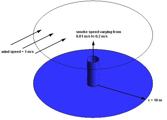
In this example, a chimney stack releases smoke that is dispersed into the atmosphere with an oncoming side wind of 1 m/s. The turbulence will be set to intensity and length scale with a value of 0.05, which corresponds to 5% turbulence, a medium level intensity, and with an eddy length scale value of 0.25 m. The goal of this tutorial is to model the dispersion of the smoke from the chimney stack over time. Unlike previous tutorials, which were steady-state, this example is time-dependent. Initially, no smoke is being released. Subsequently, the chimney starts to release smoke. As a postprocessing exercise, you produce an animation that illustrates how the plume of smoke develops with time.
If this is the first tutorial you are working with, it is important to review the following topics before beginning:
Create a working directory.
Ansys CFX uses a working directory as the default location for loading and saving files for a particular session or project.
Download the
circvent.zipfile here .Unzip
circvent.zipto your working directory.Ensure that the following tutorial input file is in your working directory:
CircVentMesh.gtm
Set the working directory and start CFX-Pre.
For details, see Setting the Working Directory and Starting Ansys CFX in Stand-alone Mode.
This section describes the step-by-step definition of the flow physics in CFX-Pre for a simulation with two analyses. First is a steady-state analysis with no smoke being produced by the chimney. The second analysis takes the setup for the steady-state and adapts it for a transient analysis. The results from the steady-state analysis will be used as the initial guess for the transient analysis.
In CFX-Pre, select File > New Case.
Select General and click .
Select File > Save Case As.
Set File name to
CircVent.Click .
Right-click
Meshand select Import Mesh > CFX Mesh.The Import Mesh dialog box appears.
Configure the following setting(s):
Setting
Value
File name
CircVentMesh.gtm
Click Open.
Right-click a blank area in the viewer and select Predefined Camera > Isometric View (Z up) from the shortcut menu.
In this tutorial an Additional Variable (non-reacting scalar component) will be used to model the dispersion of smoke from the vent.
Note: While smoke is not required for the steady-state simulation, including it here prevents you from having to set up time value interpolation in the transient analysis.
From the menu bar, select Insert > Expressions, Functions and Variables > Additional Variable.
Set Name to
smoke.Click .
Set Variable Type to
Volumetric.Set Units to
[kg m^-3].Click .
The existing analysis will be set up as steady-state.
To rename the existing analysis:
From the Outline tree, right-click
Simulation>Flow Analysis 1and click Rename.Rename the analysis to
Steady State Analysis.
You will create a fluid domain that includes support for smoke as an Additional Variable.
Select Insert > Domain from the menu bar, or click Domain
 ,
then set the name to
,
then set the name to CircVentand click .Configure the following setting(s):
Tab
Setting
Value
Basic Settings
Location and Type
> Location
B1.P3
Fluid and Particle Definitions
Fluid 1
Fluid and Particle Definitions
> Fluid 1
> Material
Air at 25 C
Domain Models
> Pressure
> Reference Pressure
0 [atm]
Fluid Models Heat Transfer
> Option
None
Turbulence
> Option
k-Epsilon
Additional Variable Models
> Additional Variable
smoke
Additional Variable Models
> Additional Variable
> smoke
(Selected)
Additional Variable Models
> Additional Variable
> smoke
> Kinematic Diffusivity
(Selected)
Additional Variable Models
> Additional Variable
> smoke
> Kinematic Diffusivity
> Kinematic Diffusivity
1.0E-5 [m^2 s^-1] [a]
Click .
This is an example of external flow, since fluid is flowing over an object and not through an enclosure such as a pipe network (which would be an example of internal flow). In external flow problems, some inlets will be made sufficiently large that they do not affect the CFD solution. However, the length scale values produced by the Default Intensity and AutoCompute Length Scale option for turbulence are based on inlet size. They are appropriate for internal flow problems and particularly, cylindrical pipes. In general, you need to set the turbulence intensity and length scale explicitly for large inlets in external flow problems. If you do not have a value for the length scale, you can use a length scale based on a typical length of the object over which the fluid is flowing. In this case, you will choose a turbulence length scale that is one-tenth of the diameter of the vent.
For parts of the boundary where the flow direction changes, or is unknown, an opening boundary can be used. An opening boundary allows flow to both enter and leave the fluid domain during the course of the analysis.
You will create the inlet boundary with velocity components set consistently with the problem description.
Select Insert > Boundary from the menu bar or click Boundary
 .
.Set Name to
Wind.Click .
Configure the following setting(s):
Tab
Setting
Value
Basic Settings
Boundary Type
Inlet
Location
Wind
Boundary Details
Mass And Momentum
> Option
Cart. Vel. Components
Mass and Momentum
> U
1 [m s^-1]
Mass and Momentum
> V
0 [m s^-1]
Mass and Momentum
> W
0 [m s^-1]
Turbulence
> Option
Intensity and Length Scale
Turbulence
> Fractional Intensity
0.05 [a]
Turbulence
> Eddy Length Scale
0.25 [m] [a]
Additional Variables
> smoke
Value
Additional Variables
> smoke
> Add. Var. Value
0 [kg m^-3] [b]
Click .
Note: The boundary marker vectors used to display boundary conditions (inlets, outlets, openings) are normal to the boundary surface regardless of the actual direction specification. To plot vectors in the direction of flow, select Boundary Vector under the Plot Options tab for the inlet boundary, and on the Labels and Markers Options tab (accessible from Case Options > Labels and Markers on the Outline tree view), ensure that Settings > Show Boundary Markers is selected and Show Inlet Markers is cleared.
You will create an opening boundary with pressure and flow direction specified. If fluid enters the domain through the opening, it should have turbulence intensity and length scale, as well as smoke concentration, set to the same values as for the inlet.
Select Insert > Boundary from the menu bar or click Boundary
.Set Name to
Atmosphere.Click .
Configure the following setting(s):
Tab
Setting
Value
Basic Settings
Boundary Type
Opening
Location
Atmosphere
Boundary Details
Mass And Momentum
> Option
Opening Pres. and Dirn
Mass and Momentum
> Relative Pressure
0 [Pa]
Flow Direction
> Option
Normal to Boundary Condition
Turbulence
> Option
Intensity and Length Scale
Turbulence
> Fractional Intensity
0.05
Turbulence
> Eddy Length Scale
0.25 [m]
Additional Variables
> smoke
> Option
Value
Additional Variables
> smoke
> Add. Var. Value
0 [kg m^-3]
Click .
You will create the vent inlet boundary with a normal velocity of 0.01 m/s as prescribed in the problem description and no smoke release. The turbulence level for the inlet vent will be determined from turbulence intensity and eddy viscosity ratio.
Select Insert > Boundary from the menu bar or click Boundary
.Set Name to
Vent.Click .
Configure the following setting(s):
Tab
Setting
Value
Basic Settings
Boundary Type
Inlet
Location
Vent
Boundary Details
Mass And Momentum
> Normal Speed
0.01 [m s^-1]
Turbulence
> Option
Intensity and Eddy Viscosity Ratio
Turbulence
> Fractional Intensity
0.05
Turbulence
> Eddy Viscosity Ratio
10
Additional Variables
> smoke
> Option
Value
Additional Variables
> smoke
> Add. Var. Value
0 [kg m^-3]
Click .
For this tutorial, the automatic initial values are suitable. Review and apply the default settings:
Click Global Initialization
 .
.Review the settings for velocity, pressure, turbulence and the smoke.
Click .
CFX-Solver has the ability to calculate physical time step size
for steady-state problems. If you do not know the time step size to
set for your problem, you can use the Auto Timescale option.
Click Solver Control
 .
.Configure the following setting(s):
Tab
Setting
Value
Basic Settings
Convergence Control
> Max. Iterations
75
Note that Convergence Control > Fluid Timescale Control > Timescale Control is set to
Auto Timescale.Click .
In this part of the tutorial, you will duplicate the steady-state analysis and adapt it to set up a transient flow analysis in CFX-Pre.
In the Outline tree view, right-click
Simulation>Steady State Analysisand select Duplicate.Right-click
Simulation>Copy of Steady State Analysisand select Rename.Rename the analysis to
Transient Analysis.
In this step you will set the new analysis to a type of transient. Later, you will set the concentration of smoke for the transient analysis to rise asymptotically to its final concentration with time, so it is necessary to ensure that the interval between the time steps is smaller at the beginning of the simulation than at the end.
In the Outline tree view, ensure that
Simulation>Transient Analysisis expanded.Right-click
Simulation>Transient Analysis>Analysis Typeand select Edit.Configure the following setting(s):
Tab
Setting
Value
Basic Settings
Analysis Type
> Option
Transient
Analysis Type
> Time Duration
> Option
Total Time
Analysis Type
> Time Duration
> Total Time
30 [s]
Analysis Type
> Time Steps
> Timesteps
4*0.25, 2*0.5, 2*1.0, 13*2.0 [s] [a]
Analysis Type
> Initial Time
> Option
Automatic with Value
Analysis Type
> Initial Time
> Time
0 [s]
Click .

The only boundary condition that needs altering for the transient
analysis is the Vent boundary condition. In the
steady-state calculation, this boundary had a small amount of air
flowing through it. In the transient calculation, more air passes
through the vent and there is a time-dependent concentration of smoke
in the air. This is initially zero, but builds up to a larger value.
The smoke concentration will be specified using the CFX Expression
Language.
In the Outline tree view, ensure that
Simulation>Transient Analysis>CircVentis expanded.Right-click
Simulation>Transient Analysis>CircVent>Ventand select Edit.Configure the following setting(s):
Tab
Setting
Value
Boundary Details
Mass And Momentum
> Normal Speed
0.2 [m s^-1]
Leave the Vent details view open for now.
You are going to create an expression for smoke concentration. The concentration is zero for time t=0 and builds up to a maximum of 1 kg m^-3.
Create a new expression by selecting Insert > Expressions, Functions and Variables > Expression from the menu bar. Set the name to
TimeConstant.Configure the following setting(s):
Name
Definition
TimeConstant
3 [s]
Click to create the expression.
Create the following expressions with specific settings, remembering to click after each is defined:
Name
Definition
FinalConcentration
1 [kg m^-3]
ExpFunction
FinalConcentration*abs(1-exp(-t/TimeConstant)) [a]
When entering this function, you can select most of the required items by right-clicking in the Definition window in the Expression details view instead of typing them. The names of the existing expressions are under the Expressions menu. The exp and abs functions are under Functions > CEL. The variable t is under Variables.
Note: The
absfunction takes the modulus (or magnitude) of its argument. Even though the expression (1- exp (-t/TimeConstant)) can never be less than zero, the abs function is included to ensure that the numerical error in evaluating it near to zero will never make the expression evaluate to a negative number.
Next, you will visualize how the concentration of smoke issued from the vent varies with time.
Double-click
ExpFunctionin the Expressions tree view.Configure the following setting(s):
Tab
Setting
Value
Plot
t
(Selected)
t
> Start of Range
0 [s]
t
> End of Range
30 [s]
Click Plot Expression.
The button name then changes to Define Plot, as shown.
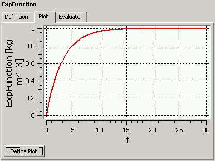
As can be seen, the smoke concentration rises to its asymptotic value reaching 90% of its final value at around 7 seconds.
Click the Boundary: Vent tab.
In the next step, you will apply the expression
ExpFunctionto the additional variablesmokeas it applies to theTransient AnalysisboundaryVent.Configure the following setting(s):
Tab
Setting
Value
Boundary Details
Additional Variables
> smoke
> Option
Value
Additional Variables
> smoke
> Add. Var. Value
ExpFunction [a]
Click .
When the Transient Analysis is run, the
initial values to the CFX-Solver will be taken from the results of the Steady State Analysis. The steady state and transient
analyses will be sequenced by setting up the configurations of these
analyses in a subsequent step. For the moment, you can leave all of
the initialization data set for the Transient Analysis to Automatic and the initial values will be
read automatically from the Steady State Analysis results. Therefore, there is no need to revisit the initialization
settings.
In the Outline tree view, ensure that
Simulation>Transient Analysis>Solveris expanded.Right-click
Simulation>Transient Analysis>Solver>Solver Controland select Edit.Set Convergence Control > Max. Coeff. Loops to
3.Leave the other settings at their default values.
Click to set the solver control parameters.
To enable results to be viewed at different time steps, it is necessary to create transient results files at specified times. The transient results files do not have to contain all solution data. In this step, you will create minimal transient results files.
In the Outline tree view, double-click
Simulation>Transient Analysis>Solver>Output Control.Click the Trn Results tab.
In the Transient Results tree view, click Add new item
 , set Name to
 Transient Results 1, and click OK.Configure the following setting(s) of
Transient Results 1:Click .
In the Transient Results tree view, click Add new item
set Name to Transient Results 2, and click OK.This creates a second transient results object. Each object can result in the production of many transient results files.
Configure the following setting(s) of
Transient Results 2:Setting
Value
Option
Selected Variables
Output Variables List
Pressure, Velocity, smoke
Output Frequency
> Option
Time Interval
Output Frequency
> Time Interval
4 [s] [a]
Click .

With two types of analysis for this simulation, configuration control is used to sequence these analyses.
To set up the Steady State Analysis so
that it will start at the beginning of the simulation:
In the Outline tree view, ensure that
Simulation Controlis expanded.Right-click
Simulation Control>Configurationsand select Insert > Configuration.Set Name to
Steady State.Click .
Configure the following setting(s):
Tab
Setting
Value
General Settings
Flow Analysis
Steady State Analysis
Activation Conditions
> Activation Condition 1
> Option
Start of Simulation
Click .
To set up the Transient Analysis so that
it will start upon the completion of the Steady State Analysis:
Right-click
Simulation Control>Configurationsand select Insert > Configuration.Set Name to
Transient.Click .
Configure the following setting(s):
Tab
Setting
Value
General Settings
Flow Analysis
Transient Analysis
Activation Conditions
> Activation Condition 1
> Option
End of Configuration
Activation Conditions
> Activation Condition 1
> Configuration Name
Steady State
Run Definition
Configuration Execution Control
Selected
Initial Values
Initial Values Specification
Selected
Initial Values Specification
> Initial Values
> Initial Values 1
> Option
Configuration Results
Initial Values Specification
> Initial Values
> Initial Values 1
> Configuration Name
Steady State
Click .
In the Outline tree view, right-click
Simulation Controland select Write Solver Input File.Configure the following setting(s):
Setting
Value
File of type
CFX-Solver Input Files (*.mdef)
File name
CircVent.mdef
Click .
This will create
CircVent.mdefas well as a directory namedCircVentthat containsSteadyState.cfgandTransient.cfg.Quit CFX-Pre, saving the case (
.cfx) file.
You can obtain a solution to the steady-state and transient configurations by using the following procedure.
Start CFX-Solver Manager.
From the menu bar, select File > Define Run.
Configure the following setting(s):
Setting
Value
Solver Input File
CircVent.mdef
Edit Configuration
Global Settings
Click Start Run.
CFX-Solver Manager will start with the solution of the steady-state configuration.
In the Workspace drop-down menu, select
SteadyState_001. The residual plots for six equations will appear: U - Mom, V - Mom, W - Mom, P - Mass, K-TurbKE, and E-Diss.K (the three momentum conservation equations, the mass conservation equation and equations for the turbulence kinetic energy and turbulence eddy dissipation). The Momentum and Mass tab contains four of the plots and the other two are under Turbulence Quantities. The residual for the smoke equation is also plotted but registers no values since it is not initialized.Upon the successful completion of the steady-state configuration, the solution of the transient configuration starts automatically. Notice that the text output generated by the CFX-Solver in the
Run Transient 001Workspace will be more than you have seen for steady-state problems. This is because each time step consists of several inner (coefficient) iterations. At the end of each time step, information about various quantities is printed to the text output area. The residual for the smoke equation is now plotted under the Additional Variables tab.Upon the successful completion of the combined steady-state and transient configurations, ensure that the check box beside Post-Process Results is cleared and click to close the message indicating the successful completion of the simulation.
In the CFX-Solver Manager, set Workspace to
Run CircVent 001.From the menu bar, select Tools > Post-Process Results.
On the Start CFD-Post dialog box, select Shut down CFX-Solver Manager and click .
In this part of the tutorial, you will:
Create an isosurface to illustrate the pattern of smoke concentration.
View results at different time steps.
Animate the results to view the dispersion of smoke from the vent over time.
Save the animation as an MPEG file.
Use volume rendering to show the visibility of smoke with its transparency.
An isosurface is a surface of constant value of a variable.
For instance, it could be a surface consisting of all points where
the velocity is 1 [m s^-1]. In this case, you are going
to create an isosurface of smoke concentration
(smoke is the Additional Variable that you specified
earlier).
In CFD-Post, right-click a blank area in the viewer and select Predefined Camera > Isometric View (Z up).
This ensures that the view is set to a position that is best suited to display the results.
From the menu bar, select Insert > Location > Isosurface, or under Location on the toolbar, click Isosurface.
Click to accept the default name.
Configure the following setting(s):
Tab
Setting
Value
Geometry
Variable
smoke
Value
0.005 [kg m^-3]
Click .
A bumpy surface is displayed, showing the smoke emanating from the vent.
The surface is rough because the mesh is coarse. For a smoother surface, you would re-run the problem with a smaller mesh length scale.
The surface will be a constant color because the default settings on the Color tab were used.
When Color Mode is set to either
ConstantorUse Plot Variablefor an isosurface, the isosurface is displayed in one color.
In Geometry, experiment by changing the Value setting so that you can see the shape of the plume more clearly.
Zoom in and rotate the geometry, as required.
When you have finished, set Value to
0.002 [kg m^-3].Right-click a blank spot in the viewer and select Predefined Camera > Isometric View (Z up).
When CFD-Post is loaded, the results that are immediately available are those at the final time step; in this case, at t = 30 s (this is nominally designated Final State). The Timestep Selector shows the Configuration, the step of the Simulation, the Step (outer loop) number, the Time (simulated time in seconds) of the configuration and the Type of results file that was saved at that time step for the configuration. You can see that Partial results files were saved (as requested in CFX-Pre) for all time steps in the transient configuration except for the last one.
Click Timestep Selector
 .
.Load the results for a Time value of 2 s by double-clicking the appropriate row in the Timestep Selector.
After a short pause, the Loaded Timestep (located just below the title bar of the Timestep Selector) will be updated with the new time step number.
Load the time value of 4 s using the Timestep Selector.
The smoke has now spread out even more, and is being carried by the wind.
Double-click some more time values to see how the smoke plume grows with time.
Finish by loading a time value of 12 s.
You can produce titled image output from CFD-Post.
First, you will add text to the viewer so that the printed output has a title.
Select Insert > Text from the menu bar or click Create text
 .
.Click to accept default name.
In the Text String box, enter the following text.
Isosurface showing smoke concentration of 0.002 kg/m^3 after
Note: Further text will be added at a later stage to complete this title.
Set Type to
Time Value.In the text line, note that
<aa>has been added to the end. This is where the time value will be placed.Click to create the title.
Click the Location tab to modify the position of the title.
The default settings for text objects center text at the top of the screen. To experiment with the position of the text, change the settings on the Location tab.
Under the Appearance tab, change Color Mode to
User Specifiedand select a new color.Click .
CFD-Post can save images in several different formats. In this section you will save an image in JPEG format.
Select File > Save Picture, or click Save Picture
 .
.Set Format to
JPEG.Click Browse
 next
to the File data box.
next
to the File data box.Browse to the directory where you want the file saved.
Enter a name for the JPEG file.
Click to set the file name and directory.
This sets the path and name for the file.
To save the file, click on the Save Picture dialog box.
To view the file or make a hard copy, use an application that supports JPEG files.
Turn off the visibility of the text object to hide it.
You can generate an MPEG file to show the transient flow of the plume of smoke. To generate a movie file, you use the Animation dialog box.
In the Timestep Selector, ensure that a time value of 0 s is loaded.
Click Animation
 .
.The Animation dialog box appears.
Set Type to Timestep Animation.
Position the geometry so that you will be able to see the plume of smoke.
Click More Animation Options
 to show more animation settings.
Ensure that the Repeat forever button
 next to Repeat is not selected
(not depressed).
next to Repeat is not selected
(not depressed).Select Save Movie.
Set Format to
MPEG1.Click Browse
next
to Save Movie.Set File name to
CircVent.mpg.If required, set the path location to a different directory.
Click .
The movie file name (including path) has been set, but the animation has not yet been produced.
Click Play the animation
 .
.The movie will be created as the animation proceeds.
This will be slow, because for each time step results will be loaded and objects will be created.
To view the movie file, you need to use a viewer that supports the MPEG format.
Note: To explore additional animation options, click the Options button. On the Advanced tab of Animation Options, there is a check box called Save Frames As Image Files. By selecting this check box, the JPEG or PPM files used to encode each frame of the movie will persist after movie creation; otherwise, they will be deleted.
The final time step has the greatest dispersion of smoke, so you will load only that time step, then view the smoke using the Volume Rendering feature.
Select File > Load Results.
In the Load Results File dialog box, select Load only the last results (the other default settings should remain unchanged) and ensure that File name is set to CircVent_001.mres. Click Open.
Note: A warning message appears. Click .
If necessary, right-click a blank spot in the viewer and select Predefined Camera > Isometric View (Z up).
In the Outline tree view, clear Isosurface 1 and Text 1.
Select Insert > Volume Rendering and set the Name to be
SmokeVolume.In the details view, set the following values:
Tab
Setting
Value
Geometry
Variable
smoke
Resolution
50
Transparency
.2
Color
Mode
Variable
Variable
smoke
Color Map
Greyscale
Click .
When you have finished, quit CFD-Post.