


This tutorial includes:
In this tutorial you will learn about:
Setting up an immersed solids domain.
Applying a counter-rotating wall boundary.
Monitoring an expression during a solver run.
Creating an XY-transient chart in CFD-Post.
Creating a keyframe animation.
Component | Feature | Details |
|---|---|---|
CFX-Pre | User Mode | General mode |
Domain Type | Immersed Solid | |
Fluid Domain | ||
Analysis Type | Transient | |
Fluid Type | Continuous Fluid | |
Boundary Conditions | Inlet Boundary | |
Outlet Boundary | ||
Domain Interface | Fluid Fluid | |
CFD-Post | Chart | Mass Flow Rate |
Animation | Keyframe |
In this tutorial, you will simulate a gear pump that drives a flow of water. This tutorial makes use of the Immersed Solids capability of Ansys CFX in order to model a solid that moves through a fluid.
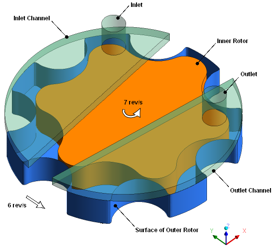
The outlet has an average relative static pressure of 1 psi; the relative total pressure at the inlet is 0 psi. The inner rotor (gear) rotates at a rate of 7 revolutions per second; the outer rotor rotates at 6 revolutions per second. The diameter of the fluid region between the rotors is approximately 7.3 cm.
You will use an immersed solid domain to model the inner rotor, a rotating fluid domain to model the water immediately surrounding the inner rotor, and a stationary fluid domain to model the water in the inlet and outlet channels. To model the stationary pump housing (not shown in the figure), you will apply a counter-rotating wall condition to the top (high Z) surface of the rotating fluid domain, on the non-overlap portion (which lies between the inlet and outlet channels). To model the upper surfaces of the teeth of the outer rotor, you will apply a rotating wall condition on the non-overlap portions of the lower (low Z) surfaces of the inlet and outlet chambers.
The following conditions will be met to promote the establishment of a cyclic flow pattern:
The mesh of the rotating domain should be rotationally periodic so that it looks the same after each (outer) rotor tooth passes.
The mesh on the outer boundary of the immersed solid domain should be rotationally periodic so that it looks the same after each (inner) rotor tooth passes. (The mesh inside the immersed solid domain has no effect in this tutorial.)
An integer number of time steps should pass as one rotor tooth passes.
If this is the first tutorial you are working with, it is important to review the following topics before beginning:
Create a working directory.
Ansys CFX uses a working directory as the default location for loading and saving files for a particular session or project.
Download the
immersed_solid.zipfile here .Unzip
immersed_solid.zipto your working directory.Ensure that the following tutorial input file is in your working directory:
ImmersedSolid.gtm
Set the working directory and start CFX-Pre.
For details, see Setting the Working Directory and Starting Ansys CFX in Stand-alone Mode.
This section describes the step-by-step definition of the flow physics in CFX-Pre for a steady-state simulation.
In CFX-Pre, select File > New Case.
Select General and click .
Select File > Save Case As.
Under File name, type
ImmersedSolid.Click .
Right-click
Meshand select Import Mesh > CFX Mesh.The Import Mesh dialog box appears.
Configure the following setting(s):
Setting
Value
File name
ImmersedSolid.gtm
Click Open.
Next, you will create an expression defining the time step size for this transient analysis. One tooth of the inner (or outer) rotor passes every 1/42 s. Choose a time step that resolves this motion in 30 intervals.
From the main menu, select Insert > Expressions, Functions and Variables > Expression.
In the Insert Expression dialog box, type
dt.Click .
Set Definition, to
(1/42)[s]/30.Click Apply to create the expression.
Next, you will create an expression defining the total simulation time. Make the simulation run long enough for 3 rotor teeth to pass: 3/42 s. This will give the solution time to establish a periodic nature.
Create an expression called
total time.Set Definition to
(3/42)[s].Click Apply.
Define the simulation as transient, using the expressions you created earlier.
Under the Outline tab, edit Analysis Type
 .
. Configure the following setting(s):
Tab
Setting
Value
Basic Settings
Analysis Type
> Option
Transient
Analysis Type
> Time Duration
> Option
Total Time
Analysis Type
> Time Duration
> Total Time
total time [a]
Analysis Type
> Time Steps
> Option
Timesteps
Analysis Type
> Time Steps
> Timesteps
dt
Analysis Type
> Initial Time
> Option
Automatic with Value
Analysis Type
> Initial Time
> Time
0 [s]
Click .

This simulation requires three domains: two fluid domains and one immersed solid domain. First you will create an immersed solid domain.
Create the immersed solid domain as follows:
Select Insert > Domain from the main menu, or click Domain
 .
.In the Insert Domain dialog box, set the name to
ImmersedSolidand click .Configure the following setting(s):
Tab
Setting
Value
Basic Settings
Location and Type
> Location
Inner Rotor
Location and Type
> Domain Type
Immersed Solid
Location and Type
> Coordinate Frame
Coord 0
Domain Models
> Domain Motion
> Option
Rotating
Domain Models
> Domain Motion
> Angular Velocity
7 [rev s^-1]
Domain Models
> Domain Motion
> Axis Definition
> Option
Two Points
Domain Models
> Domain Motion
> Axis Definition
> Rotation Axis From
0.00383, 0, 0
Domain Models
> Domain Motion
> Axis Definition
> Rotation Axis To
0.00383, 0, 1
Click .
Create the stationary fluid domain according to the problem description:
Create a new domain named
StationaryFluid.Configure the following setting(s):
Tab
Setting
Value
Basic Settings
Location and Type
> Location
Channels
Location and Type
> Domain Type
Fluid Domain
Location and Type
> Coordinate Frame
Coord 0
Fluid and Particle Definitions
Fluid 1
Fluid and Particle Definitions
> Fluid 1
> Option
Material Library
Fluid and Particle Definitions
> Fluid 1
> Material
Water
Fluid and Particle Definitions
> Fluid 1
> Morphology
> Option
Continuous Fluid
Domain Models
> Pressure
> Reference Pressure
0 [psi]
Domain Models
> Buoyancy Models
> Option
Non Buoyant
Domain Models
> Domain Motion
> Option
Stationary
Domain Models
> Mesh Deformation
> Option
None
Fluid Models
Heat Transfer
> Option
None
Turbulence
> Option
k-Epsilon
Turbulence
> Wall Function
Scalable
Combustion
> Option
None
Thermal Radiation
> Option
None
Initialization
Domain Initialization
(Selected)
Domain Initialization
> Initial Conditions
> Velocity Type
Cartesian
Domain Initialization
> Initial Conditions
> Cartesian Velocity Components
> Option
Automatic with Value
Domain Initialization
> Initial Conditions
> Cartesian Velocity Components
> U
0 [m s^-1]
Domain Initialization
> Initial Conditions
> Cartesian Velocity Components
> V
0 [m s^-1]
Domain Initialization
> Initial Conditions
> Cartesian Velocity Components
> W
0 [m s^-1]
Domain Initialization
> Initial Conditions
> Static Pressure
> Option
Automatic with Value
Domain Initialization
> Initial Conditions
> Static Pressure
> Relative Pressure
1 [psi] * step(-y/1 [cm]) [a]
Domain Initialization
> Initial Conditions
> Turbulence
> Option
Medium (Intensity = 5%)
Click .
Create the rotating fluid domain according to the problem description:
In the Outline tree view, right-click
Simulation>Flow Analysis 1>StationaryFluidand select Duplicate.Right-click
Simulation>Flow Analysis 1>Copy of StationaryFluidand select Rename.Rename the domain to
RotatingFluid.Edit
RotatingFluid.Configure the following setting(s):
Tab
Setting
Value
Basic Settings
Location and Type
> Location
Gear Chamber
Domain Models
> Domain Motion
> Option
Rotating
Domain Models
> Domain Motion
> Angular Velocity
6 [rev s^-1]
Domain Models
> Domain Motion
> Axis Definition
> Option
Coordinate Axis
Domain Models
> Domain Motion
> Axis Definition
> Rotation Axis
Global Z
Click .
Add a domain interface that connects the StationaryFluid and RotatingFluid domains:
Click Insert > Domain Interface from the main menu or click Domain Interface
 .
.Accept the default domain interface name and click .
Configure the following setting(s):
Tab
Setting
Value
Basic Settings
Interface Type
Fluid Fluid
Interface Side 1
> Domain (Filter)
StationaryFluid
Interface Side 1
> Region List
Channel Side
Interface Side 2
> Domain (Filter)
RotatingFluid
Interface Side 2
> Region List
Chamber Side
Interface Models
> Option
General Connection
Interface Models
> Frame Change/Mixing Model
> Option
Transient Rotor Stator
Interface Models
> Pitch Change
> Option[i]
None
Additional Interface Models
Mass and Momentum
> Option
Conservative Interface Flux
Mass and Momentum
> Interface Model
> Option
None
Mesh Connection
Mesh Connection Method
> Mesh Connection
> Option
GGI
Click .
Apply a counter-rotating no-slip wall condition to the non-overlap portion of the domain interface on the rotating domain side, because this surface represents part of the stationary housing of the pump.
Edit
RotatingFluid>Domain Interface 1 Side 2.If this object does not appear in the tree view, then edit
Case Options>General, select Show Interface Boundaries in Outline Tree, and click .Configure the following setting(s):
Tab
Setting
Value
Nonoverlap Conditions
Nonoverlap Conditions
(Selected)
Nonoverlap Conditions
> Mass and Momentum
> Option
No Slip Wall
Nonoverlap Conditions
> Mass and Momentum
> Wall Velocity
(Selected)
Nonoverlap Conditions
> Mass and Momentum
> Wall Velocity
> Option
Counter Rotating Wall
Click OK.
Apply a rotating no-slip wall condition to the non-overlap portions of the domain interface on the stationary domain side, because these surfaces represent faces of the rotor teeth of the outer rotor, and the latter rotates at 6 rev/s about the Z axis.
Edit
StationaryFluid>Domain Interface 1 Side 1.Configure the following setting(s):
Tab
Setting
Value
Nonoverlap Conditions
Nonoverlap Conditions
(Selected)
Nonoverlap Conditions
> Mass and Momentum
> Option
No Slip Wall
Nonoverlap Conditions
> Mass and Momentum
> Wall Velocity
(Selected)
Nonoverlap Conditions
> Mass and Momentum
> Wall Velocity
> Option
Rotating Wall
Nonoverlap Conditions
> Mass and Momentum
> Wall Velocity
> Angular Velocity
6 [rev s^-1]
Nonoverlap Conditions
> Mass and Momentum
> Wall Velocity
> Axis Definition
> Option
Coordinate Axis
Nonoverlap Conditions
> Mass and Momentum
> Wall Velocity
> Axis Definition
> Rotation Axis
Global Z
Click OK.
This section outlines the steps to create the inlet and outlet boundary conditions, as specified in the problem description.
Create a total pressure inlet at a relative pressure of 0 psi:
In the Outline tree view, right-click
StationaryFluidand select Insert > Boundary.Set Name to
inand click OK.Configure the following setting(s):
Tab
Setting
Value
Basic Settings
Boundary Type
Inlet
Location
Inlet
Boundary Details
Mass And Momentum
> Option
Total Pressure (stable)
Mass And Momentum
> Relative Pressure
0 [psi]
Flow Direction
> Option
Normal to Boundary Condition
Turbulence
> Option
Medium (Intensity = 5%)
Click .
Create an outlet with a relative average static pressure of 1 psi:
Create a boundary named
outin theStationaryFluiddomain.Configure the following setting(s):
Tab
Setting
Value
Basic Settings
Boundary Type
Outlet
Location
Outlet
Boundary Details
Mass And Momentum
> Option
Average Static Pressure
Mass And Momentum
> Relative Pressure
1 [psi]
Mass And Momentum
> Pres. Profile Blend
0.05
Pressure Averaging
> Option
Average Over Whole Outlet
Click .
Click Solver Control
 .
.Configure the following setting(s):
Tab
Setting
Value
Basic Settings
Advection Scheme
> Option
High Resolution
Transient Scheme
> Option
Second Order Backward Euler
Transient Scheme
> Timestep Initialization
> Option
Automatic
Turbulence Numerics
> Option
First Order
Convergence Control
> Min. Coeff. Loops
1
Convergence Control
> Max. Coeff. Loops
10
Convergence Control
> Fluid Timescale Control
> Timescale Control
Coefficient Loops
Convergence Criteria
> Residual Type
RMS
Convergence Criteria
> Residual Target
1.0 E −4
Click .
Set up the solver to output transient results files that record pressure, velocity, and velocity in the stationary frame, on every time step:
Click Output Control
 .
.Click the Trn Results tab.
In the Transient Results list box, click Add new item
 , set Name to
 Transient Results 1, and click OK.Configure the following setting(s) of
Transient Results 1:Setting
Value
Option
Selected Variables
File Compression
Default
Output Variables List
Pressure, Velocity, Velocity in Stn Frame
Output Boundary Flows
(Selected)
Output Boundary Flows
> Boundary Flows
All
Output Frequency
> Option
Every Timestep
Click the Monitor tab.
Select Monitor Objects.
Under Monitor Points and Expressions:
Click Add new item
.Accept the default name and click .
Set Option to
Expression.Set Expression Value to
massFlow()@in.
Click .
Click Define Run
 .
.Configure the following setting(s):
Setting
Value
File name
ImmersedSolid.def
Click .
Note: A warning message will appear due to the global warning that was mentioned earlier in Creating the Domain Interface. Click Yes.
CFX-Solver Manager automatically starts and, on the Define Run dialog box, Solver Input File is set.
If using stand-alone mode, quit CFX-Pre, saving the simulation (
.cfx) file at your discretion.
When CFX-Pre has shut down and the CFX-Solver Manager has started, obtain a solution to the CFD problem by following the instructions below:
In CFX-Solver Manager, ensure that the Define Run dialog box is displayed.
If CFX-Solver Manager is launched from CFX-Pre, the information required to perform a solver run is entered automatically in the Define Run dialog box.
Click Start Run.
The solver run begins and the progress is displayed in a split screen.
Click the User Points tab (which appears after the first time step has been computed) and monitor the value of
Monitor Point 1as the solution proceeds.Rescale the monitor plot so that you can readily see the time-periodic oscillations in mass flow that occur after the initial transient phase:
Right-click anywhere in the User Points plot and select Monitor Properties.
In the Monitor Properties: User Points dialog box, on the Range Settings tab, select Set Manual Scale (Linear).
Set the lower and upper bounds to 0.015 and 0.055 respectively.
Click OK.
Select the check box next to Post-Process Results when the completion message appears at the end of the run.
If using stand-alone mode, select the check box next to Shut down CFX-Solver Manager.
Click .
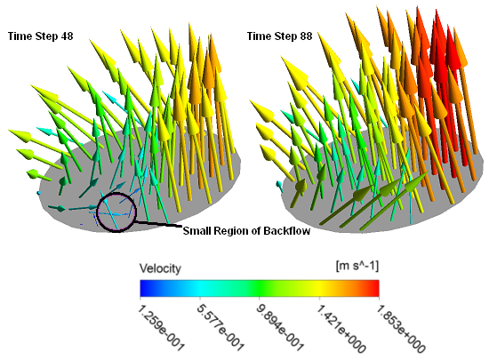
Note: During the Solver Manager run, you may observe a notice at the 47th and 48th time steps warning you that "A wall has been placed at portion(s) of an OUTLET boundary condition ... to prevent fluid from flowing into the domain." The mass flow at the inlet drops to its lowest level throughout the cycle at this point, causing a reduction in the velocity at the outlet. Because there is turbulence at the outlet, this reduced velocity allows a tiny vortex to produce a small, virtually negligible, amount of backflow at the outlet. Figure 25.1: Velocity Vectors on the Outlet shows velocity vectors at the outlet when the mass flow at the inlet is lowest (48th time step) and when the mass flow is greatest (88th time step). In the figure, you can see where this slight backflow occurs for the 48th time step.
In this section, you will generate a chart to show the mass flow rate through the machine as a function of time. You will also prepare an animation of the machine in operation, complete with velocity vectors.
During the solver run, you observed a monitor plot that showed mass flow versus time step. Here, you will make a similar plot of mass flow versus time. As you did in the monitor plot, adjust the vertical axis range to focus on the time-periodic oscillations in mass flow that occur after the initial transient phase.
When CFD-Post starts, the Domain Selector dialog box might appear. If it does, ensure that the
ImmersedSolid,RotatingFluidandStationaryFluiddomains are selected, then click OK to load the results from these domains.A dialog box will notify you that the case contains immersed solid domain. Click to continue.
Create a new chart named
Mass Flow Rate.The Chart Viewer appears.
Configure the following setting(s):
Tab
Setting
Value
General
Type
XY-Transient or Sequence
Title
Mass Flow Rate at the Inlet over Time
Click the Data Series tab.
If the Data Series list box is empty, right-click in it and select New, or click New
.Configure the following setting(s):
Tab
Setting
Value
Data Series
Series 1
(Selected)
Name
Inlet Mass Flow
Data Source
> Expression
(Selected)
Data Source
> Expression
massFlow()@in [a]
Y Axis
Axis Range
> Determine ranges automatically
(Cleared)
Axis Range
> Min
0.015
Axis Range
> Max
0.055
Click Apply.
The mass flow rate settles into a repeating pattern with a period of 1/42 s, which is the time it takes a rotor tooth to pass.
Create a slice plane and then make a vector plot on the slice plane as follows:
Click the 3D Viewer tab.
Create a new plane named
Plane 1.Configure the following setting(s):
Tab
Setting
Value
Geometry
Domains
RotatingFluid
Definition
> Method
XY Plane
Definition
> Z
0.003 [m]
Click Apply.
Turn off the visibility of
Plane 1.Create a new vector plot named
Vector 1.Configure the following setting(s):
Tab
Setting
Value
Geometry
Domains
All Domains
Definition
> Locations
Plane 1
Definition
> Sampling
Rectangular Grid
Definition
> Spacing
0.03
Definition
> Variable
Velocity
Color
Mode
Use Plot Variable
Range
User Specified
Min
0 [m s^-1]
Max
0.8 [m s^-1]
Symbol
Symbol
Arrow3D
Symbol Size
15
Normalized Symbols
(Cleared)
Click Apply.
Make the inlet and outlet visible as follows:
Edit
StationaryFluid>in.Configure the following setting(s):
Tab
Setting
Value
Render
Show Faces
(Cleared)
Show Mesh Lines
(Selected)
Show Mesh Lines
> Edge Angle
105 [degree]
Show Mesh Lines
> Line Width
2
Show Mesh Lines
> Color Mode
Default
Click Apply.
Apply the same settings to
StationaryFluid>out.
Make the inlet and outlet channels visible as follows:
Edit
StationaryFluid>StationaryFluid Default.Configure the following setting(s):
Tab
Setting
Value
Render
Show Faces
(Selected)
Show Faces
> Transparency
0.8
Show Mesh Lines
(Cleared)
Click Apply.
Make the walls of the rotating fluid domain visible as follows:
Edit
RotatingFluid>RotatingFluid Default.Configure the following setting(s):
Tab
Setting
Value
Color
Mode
Constant
Color
(White)
Render
Show Faces
(Selected)
Show Faces
> Transparency
0.0
Show Mesh Lines
(Cleared)
Click Apply.
Make the walls of the immersed solid domain visible as follows:
Edit
ImmersedSolid>ImmersedSolid Default.Configure the following setting(s):
Tab
Setting
Value
Color
Mode
Constant
Color
(Blue)
Render
Show Faces
(Selected)
Show Faces
> Transparency
0.0
Show Mesh Lines
(Cleared)
Click Apply.
Make the following other changes in preparation for the animation that you will create in the next section:
Right-click a blank area in the viewer and select Predefined Camera > View From +Z.
Rotate the view a few degrees so that you can see the 3D nature of the geometry.
Turn off the visibility of
User Locations and Plots>Wireframe.
In this section, you will generate an animation that shows the
changing velocity field on Plane 1. To take advantage
of the periodic nature of the solution, you will record a short animation
that can be played in a repeating loop in an MPEG player. Start the
animation at the 61st time step (a time
at which the flow has settled into a repeating pattern) and end it
at the 90th time step. The 60th time step corresponds with 2/42 s, and the 90th corresponds with 3/42 s; the 1/42 s interval is
the period over which the solution repeats. Because the 60th and 90th time steps look
the same, the 60th time step is omitted
to avoid having a pair of adjacent identical frames in the animation
when the latter is played in a repeating loop.
Click Timestep Selector
 and load the 61st time step.
Click Animation
 .
.The Animation dialog box appears.
Set Type to Keyframe Animation.
Click New
to create KeyframeNo1.Select
KeyframeNo1, then set # of Frames to28, then press Enter while the cursor is in the # of Frames box.Tip: Be sure to press Enter and confirm that the new number appears in the list before continuing.
Use the Timestep Selector to load the 90th time step.
In the Animation dialog box, click New
to create KeyframeNo2.Ensure that More Animation Options
 is pushed down to show more animation settings.
Select Loop.
Ensure that the Repeat forever button
 next to Repeat is not selected
(not pushed down).
next to Repeat is not selected
(not pushed down).Select Save Movie.
Set Format to
MPEG1.Click Browse
 next
to Save Movie.
next
to Save Movie.Set File name to
ImmersedSolid.mpg.If required, set the path location to a different directory.
Click .
The movie file name (including path) has been set, but the animation has not yet been produced.
Click To Beginning
 .
.This ensures that the animation will begin at the first keyframe.
After the first keyframe has been loaded, click Play the animation
 .
.The MPEG will be created as the animation proceeds.
This will be slow, since results for each time step will be loaded and objects will be created.
To view the movie file, you need to use a viewer that supports the MPEG format.
Note: To explore additional animation options, click the Options button. On the Advanced tab of the Animation Options dialog box, there is a Save Frames As Image Files check box. By selecting this check box, the JPEG or PPM files used to encode each frame of the movie will persist after movie creation; otherwise, they will be deleted.
When you have finished, quit CFD-Post.