is the turbulence kinetic energy and is defined as the variance of the fluctuations in velocity. It has dimensions of (L² T^-2); for example, m²/s². is the turbulence eddy dissipation (the rate at which the velocity fluctuations dissipate), and has dimensions of per unit time (L² T^-3); for example, m²/s³.

The - model introduces two new variables into the system of equations. The continuity equation is then:

(2–19)

and the momentum equation becomes:

(2–20)

where is the sum of body forces, is the effective viscosity accounting for turbulence, and is the modified pressure as defined in Equation 2–14.

The - model, like the zero equation model, is based on the eddy viscosity concept, so that:

(2–21)

where is the turbulence viscosity. The - model assumes that the turbulence viscosity is linked to the turbulence kinetic energy and dissipation via the relation:

(2–22)

where is a constant. For details, see List of Symbols.

The values of and come directly from the differential transport equations for the turbulence kinetic energy and turbulence dissipation rate:

(2–23)

(2–24)

where , , and are constants. For details, see List of Symbols.

and represent the influence of the buoyancy forces, which are described below. is the turbulence production due to viscous forces, which is modeled using:

(2–25)

For incompressible flow, is small and the second term on the right side of Equation 2–25 does not contribute significantly to the production. For compressible flow, is only large in regions with high velocity divergence, such as at shocks.

The term in Equation 2–25 is based on the "frozen stress" assumption [54]. This prevents the values of and becoming too large through shocks, a situation that becomes progressively worse as the mesh is refined at shocks. The parameter Compressible Production (accessible on the Advanced Control part of the Turbulence section in CFX-Pre (see Turbulence in the CFX-Pre User's Guide)) can be used to set the value of the factor in front of , the default value is 3, as shown. A value of 1 will provide the same treatment as CFX-4.

In order to avoid the build-up of turbulent kinetic energy in stagnation regions, two production limiters are available. For details, see Production Limiters.

If the full buoyancy model is being used, the buoyancy production term is modeled as:

(2–26)

and if the Boussinesq buoyancy model is being used, it is:

(2–27)

This buoyancy production term is included in the equation if the Buoyancy Turbulence option in CFX-Pre is set to Production, or Production and Dissipation. It is also included in the equation if the option is set to Production and Dissipation. is assumed to be proportional to and must be positive, therefore it is modeled as:

(2–28)

If the directional option is selected, then is modified by a factor accounting for the angle between velocity and gravity vectors:

(2–29)

Default model constants are given by:

Turbulence Schmidt Number :

Dissipation Coefficient, C₃ = 1

Directional Dissipation = Off

For omega based turbulence models, the buoyancy turbulence terms for the equation are derived from and according to the transformation .

The RNG model is based on renormalization group analysis of the Navier-Stokes equations. The transport equations for turbulence generation and dissipation are the same as those for the standard model, but the model constants differ, and the constant is replaced by the function .

The transport equation for turbulence dissipation becomes:

(2–30)

where:

(2–31)

and:

(2–32)

For details, see List of Symbols.

One of the advantages of the - formulation is the near wall treatment for low-Reynolds number computations. The model does not involve the complex nonlinear damping functions required for the - model and is therefore more accurate and more robust. A low-Reynolds - model would typically require a near wall resolution of , while a low-Reynolds number - model would require at least . In industrial flows, even cannot be guaranteed in most applications and for this reason, a new near wall treatment was developed for the - models. It allows for smooth shift from a low-Reynolds number form to a wall function formulation.

The - models assume that the turbulence viscosity is linked to the turbulence kinetic energy and turbulent frequency via the relation:

(2–33)

 

2.2.2.4.1. The Wilcox k-omega Model

The starting point of the present formulations is the - model developed by Wilcox [11]. It solves two transport equations, one for the turbulent kinetic energy, , and one for the turbulent frequency, . The stress tensor is computed from the eddy-viscosity concept.

-equation:

(2–34)

-equation:

(2–35)

In addition to the independent variables, the density, , and the velocity vector, , are treated as known quantities from the Navier-Stokes method. is the production rate of turbulence, which is calculated as in the - model Equation 2–25.

The model constants are given by:

(2–36)

(2–37)

(2–38)

(2–39)

(2–40)

The unknown Reynolds stress tensor, , is calculated from:

(2–41)

In order to avoid the build-up of turbulent kinetic energy in stagnation regions, two production limiters are available. For details, see Production Limiters.

The buoyancy production term is included in the -equation if the Buoyancy Turbulence option in CFX-Pre is set to Production or Production and Dissipation. The formulation is the same is given in Equation 2–26 and Equation 2–27.

The buoyancy turbulence terms for the -equation are derived from and according to the transformation .

The additional buoyancy term in the -equation reads:

(2–42)

Here the first term on the right hand side, which comes from the -equation, is included only if the Buoyancy Turbulence option is set to Production and Dissipation. The second term, originating from the -equation, is included with both Production and Production and Dissipation options.

If the directional option is selected, then the first term on the right hand side is modified according to Equation 2–29:

(2–43)

 

2.2.2.4.2. The Baseline (BSL) k-omega Model

The main problem with the Wilcox model is its well known strong sensitivity to freestream conditions (Menter [12]). Depending on the value specified for at the inlet, a significant variation in the results of the model can be obtained. This is undesirable and in order to solve the problem, a blending between the - model near the surface and the - model in the outer region was developed by Menter [9]. It consists of a transformation of the - model to a - formulation and a subsequent addition of the corresponding equations. The Wilcox model is thereby multiplied by a blending function and the transformed - model by a function . is equal to one near the surface and decreases to a value of zero outside the boundary layer (that is, a function of the wall distance). For details, see Wall and Boundary Distance Formulation. At the boundary layer edge and outside the boundary layer, the standard - model is therefore recovered.

Wilcox model:

(2–44)

(2–45)

Transformed model:

(2–46)

(2–47)

Now the equations of the Wilcox model are multiplied by function , the transformed - equations by a function and the corresponding - and - equations are added to give the BSL model. Including buoyancy effects the BSL model reads:

(2–48)

(2–49)

The coefficient in the buoyancy production term in Equation 2–42 and Equation 2–43 is also replaced by the new coefficient .

The coefficients of the new model are a linear combination of the corresponding coefficients of the underlying models:

(2–50)

All coefficients are listed again for completeness:

(2–51)

(2–52)

(2–53)

(2–54)

(2–55)

(2–56)

(2–57)

(2–58)

(2–59)

 

2.2.2.4.3. The Shear Stress Transport (SST) Model

The - based SST model accounts for the transport of the turbulent shear stress and gives highly accurate predictions of the onset and the amount of flow separation under adverse pressure gradients.

The BSL model combines the advantages of the Wilcox and the - model, but still fails to properly predict the onset and amount of flow separation from smooth surfaces. This deficiency is discussed in detail by Menter [9], but primarily arises because these models, which do not account for the transport of the turbulent shear stress, overpredict the eddy-viscosity. The proper transport behavior can be obtained by a limiter to the formulation of the eddy-viscosity:

(2–60)

where

(2–61)

Again is a blending function similar to , which restricts the limiter to the wall boundary layer, as the underlying assumptions are not correct for free shear flows. is an invariant measure of the strain rate.

Note that the production term of is given by:

(2–62)

This formulation differs from the standard - model.

---

Note:  In the SST model, .

---

 

2.2.2.4.3.1. Blending Functions

The blending functions are critical to the success of the method. Their formulation is based on the distance to the nearest surface and on the flow variables.

(2–63)

with:

(2–64)

where is the distance to the nearest wall, is the kinematic viscosity and:

(2–65)

(2–66)

with:

(2–67)

 

2.2.2.4.3.2. The Wall Scale Equation

During the solution of a simulation using the SST or BSL model, you will see a plot in the CFX-Solver Manager for Wall Scale. These models require the distance of a node to the nearest wall for performing the blending between - and -. Detailed information on the wall scale equation is available in Wall and Boundary Distance Formulation.

 

2.2.2.4.3.3. Modifications to SST for High Lift Devices

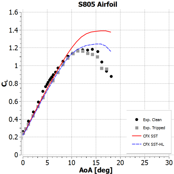
The high-lift modification for the SST turbulence model (SST-HL) is based on the observation that for numerous airfoil predictions, the SST model over-predicts the maximum lift achievable. In terms of physics, this means that the standard SST model predicts less and later flow separation from the airfoil than has been observed in experiments. The high-lift modification allows the fine tuning of the SST model for such applications. The default value (0.9) of the tuning parameter (CHL Coefficient) is optimized for a wide range of flows. Setting the parameter value to unity reverts the model back to the standard SST model. It is worth noting that all other available eddy-viscosity models lead to even stronger deviations from experimental data compared to the SST model and so do not offer an alternative to the SST-HL modification.

Figure 2.1: Example showing effect of high-lift modification on results

 

2.2.2.4.4. The Reattachment Modification (RM) Model

RANS models are designed for predicting attached and mildly separated flows. It is known that all RANS models fail in predicting the correct turbulence stress levels in large separation zones; the turbulent stresses in the separating shear layer are typically underpredicted, leading to overly large separation zones. This is often masked by the tendency of many RANS models to predict delayed separation under adverse pressure gradients compared to experimental data. As the SST model typically predicts the onset of separation with good accuracy, there is a need to introduce additional production of turbulence under such conditions. To correct the problem, the Reattachment Modification (RM) model modifies the SST model to enhance turbulence levels in the separating shear layers emanating from walls. This modification becomes less effective with increasing mesh refinement, and, as a result, is not an official amendment to the SST model. Nevertheless, the RM model is suitable for typical engineering applications, and has become especially popular for modeling turbomachinery flows.

---

Note:

• The RM model should be used only to model flows separating from smooth surfaces under the influence of adverse pressure gradients. It should not be treated as a general-purpose enhancement to the SST model, as this may suppress errors caused by poor mesh definition or inappropriate model assumptions.

• If the geometry of your case is complex, the RM model may be active in unintended regions.

• In investigating 2D cases, the RM model loses effectiveness when the mesh resolution in the boundary layer exceeds ~ 100 cells. With such significant mesh refinement, the RM model behaves like the standard SST model.

---

In free mixing layers, the ratio of turbulence production to dissipation, , has an equilibrium value of . However, the equilibrium value of is greatly exceeded in regions of large flow separation from smooth surfaces. Based on this observation, the RM model adds a source term to the right-hand side of the -equation used in the SST model. This source term, , is given by:

(2–68)

is a function that was introduced to avoid interaction between the RM model and laminar-turbulent transition models (see Ansys CFX Laminar-Turbulent Transition Models). The function is given by:

(2–69)

where represents kinematic viscosity and is an adjustable coefficient whose default value is . Note that decreasing the value of tends to decrease the effectiveness of the function .

A disadvantage of standard two-equation turbulence models is the excessive generation of turbulence energy, , in the vicinity of stagnation points. In order to avoid the build-up of turbulent kinetic energy in stagnation regions, a formulation of limiters for the production term in the turbulence equations is available.

The formulation follows Menter [9] and reads:

(2–70)

The coefficient is called Clip Factor and has a value of 10 for based models. This limiter does not affect the shear layer performance of the model, but has consistently avoided the stagnation point build-up in aerodynamic simulations.

Using the standard Boussinesq-approximation for the Reynolds stress tensor, the production term can be expressed for incompressible flow as:

(2–71)

where denotes the magnitude of the strain rate and the strain rate tensor.

Kato and Launder [128] noticed that the very high levels of the shear strain rate in stagnation regions are responsible for the excessive levels of the turbulence kinetic energy. Because the deformation near a stagnation point is nearly irrotational, that is the vorticity rate is very small, they proposed the following replacement of the production term:

(2–72)

where denotes the magnitude of the vorticity rate and the vorticity tensor. In a simple shear flow, and are equal. Therefore, formulation recovers in such flows, as seen in the first parts of Equation 2–71 and Equation 2–72.

The production limiters described above are available for the two ε based turbulence models and for the (k,)-, BSL- and SST-turbulence models. They are available in the Advanced Control settings of the Turbulence Model section in CFX-Pre. For details, see Turbulence: Option in the CFX-Pre User's Guide. The allowed options of the production limiter are Clip Factor and Kato Launder.

One weakness of the eddy-viscosity models is that these models are insensitive to streamline curvature and system rotation. Based on the work of Spalart and Shur [191] a modification of the production term has been derived to sensitize the standard two-equation models to these effects [192]. The empirical function suggested by Spalart and Shur [191] to account for these effects is defined by

(2–73)

It is used as a multiplier of the production term and has been limited in Ansys CFX in the following way:

(2–74)

where

and

The original function is limited in the range from 0.0 corresponding, for example, to a strong convex curvature (stabilized flow, no turbulence production) up to 1.25 (for example, strong concave curvature, enhanced turbulence production). The lower limit is introduced for numerical stability reasons, whereas the upper limit is needed to avoid overgeneration of the eddy viscosity in flows with a destabilizing curvature/rotation. The specific limiter 1.25 provided a good compromise for different test cases that have been considered with the SST model (for example, flow through a U-turn, flow in hydrocyclone, and flow over a NACA 0012 wing tip vortex [192]). The scaling coefficient has been introduced to enable you to influence the effect of the curvature correction if needed for a specific flow. The default value of this scaling coefficient is 1.0 and can be changed on the Fluid Models tab of the Domain details view in CFX-Pre.

Assuming that all the variables and their derivatives are defined with respect to the reference frame of the calculation, which is rotating with a rate , the arguments and of the function are defined in the following way:

(2–75)

(2–76)

where the first term in brackets is equivalent to the 2nd velocity gradient (in this case the Lagrangian derivative of the strain rate tensor) and the 2nd term in the brackets is a measure of the system rotation. The strain rate and vorticity tensor are defined, respectively, using Einstein summation convention as

(2–77)

(2–78)

where

and, where

are the components of the Lagrangian derivative of the strain rate tensor.

Finally, based on the performed tests, the empirical constants , and involved in Equation 2–73 are set equal to 1.0, 2.0, and 1.0, respectively.

This curvature correction is available for and -based eddy-viscosity turbulence models (, RNG , -, BSL, SST) as well as the DES-SST and SAS-SST turbulence models.