


The following topics are discussed:
If confronted with a new application, it is prudent to ensure that the turbulence model intended to be used is validated for this type of flows – or at least for the underlying flow features observed. Ideally, one would start with a validation study of a similar case for which experimental data are available and optimize the CFD set-up:
Geometry
Represent geometry as closely as possible – small simplifications in geometry can sometimes have large effects on the solution.
Avoid overly tight domains – try to place inlets in regions of well-defined flow and avoid outlets in regions of strong non-equilibrium flow dynamics, especially separation/backflow zones.
Conditions
Select correct physical properties for density, viscosity, …
Ensure correct representation of flow physics (rotating systems, porous media, …).
Optimal grid (see Mesh Resolution Requirements)
Select an optimal grid topology for given flows.
Ensure fine resolution of wall boundary layers (see Fully Turbulent Boundary Layers).
Perform simulations on successively refined grids until the solution no longer changes.
Boundary conditions
Match experimental/application boundary conditions closely.
Avoid inflow at outlets. Often the outlet flow can be accelerated through contraction of the domain in this region to avoid backflow.
Numerics
Decide on steady versus unsteady settings (see Steady vs Unsteady vs Convergence).
Use 2nd order numerics if possible, also for the turbulence equations.
Do not use small under-relaxation factors (URF). Small values can slow down convergence. The selection of optimal URF is as a balance between convergence speed and robustness. Default values tend to be on the conservative side towards robustness.
Turbulence model
Compare different models or modify GEKO coefficients and establish if the flow is sensitive to model changes.
Select models/coefficients which are best calibrated for the given application – or which match best the validation case at hand.
Optimize GEKO coefficients if indicated by experimental data.
Decide if additional terms need to be activated
Curvature Correction.
Corner Correction.
Rough walls.
Buoyancy.
…
Run case in automated/scripted way to avoid user errors during set-up and post-processing.
Test solution sensitivity to any arbitrary assumptions made above by variation of such parameters.
The process outlined cannot be followed in all industrial CFD projects. However, it is helpful to recall what an optimal process would look like and be aware of any shortcuts taken. Experience shows that many CFD errors result from non-optimal set-ups and meshes and not from deficiencies of the turbulence model. The most common source of error being under-resolved meshes or non-converged solutions.
The first question to consider before starting a RANS simulation is if the flow is steady or unsteady. As all turbulent flows are inherently unsteady in a physical sense, the question more precisely is if the flow is steady in the framework of RANS modeling. This might be one of the most difficult questions to answer a priori. In addition, the answer to this question can depend on the RANS model selected. RANS models that predict large zones of flow separation will be more likely to develop unsteady solutions than models that predict small or no separation zones. Often the models that predict larger separation zones are closer to the experimental data.
For cases where unsteadiness is imposed from outside, like flows with moving geometries, or unsteady boundary conditions, the situation is clear. However, there are also many flow scenarios where the set-up is 'steady', but where the flow still exhibits unsteady characteristics:
Vortex shedding behind bluff bodies.
Meandering/precessing Vortex (e.g. combustion chamber).
Rotating stall in axial turbomachines.
…
If a steady state solution is expected, the usual strategy is to set numerics to 'steady conditions' and run the case. If residuals converge 'deeply' a steady solution is achieved. Unfortunately, the question 'How deep is enough?' cannot easily be answered. While in some cases, three orders of magnitude are enough, whereas other cases might require 4-6 orders. It is therefore recommended to display monitor quantities at monitor points which are sensitive to solution convergence. One can also display distributions (e.g. xy-plots, Contour plots) of quantities during the simulation. A case in point would be to display the wall shear-stress in a cut of the geometry to judge if the solution has settled down. This is particularly important in cases where a transition model is employed as laminar-turbulent fronts tend to settle down slowly.
Unfortunately, in many complex applications, 'deep' convergence cannot be achieved, as there will invariably be small regions, where the solution might not fully settle down, partly for physical and partly for numerical or mesh quality reasons.
To judge the steadiness of the simulation in such scenarios, it is again recommended to set monitor points and plot them during the solution. This can be global parameters, like lift or drag forces, pressure drop between inlet and outlet, massflow etc. and/or local quantities like primary solution variables (u,p,T,…) at specific locations. These locations should be placed in regions of high flow complexity and the highest likelihood of convergence problems. In cases where either the residuals, or the monitor points do not settle down to an acceptable level, it is recommended to switch to unsteady mode and continue the simulation. There are cases, where switching to unsteady mode helps to converge to steady state. If this is not the case, users must decide if the unsteadiness is of relevance, or just a small local disturbance without impact on the simulation outcome. If the unsteadiness is important, then time-mean values can only be obtained by running the simulation unsteady and averaging during run-time. It can also help to create animations to understand the cause and nature of unsteady behavior.
In a worst-case scenario, a steady state set-up can force the solution into an incorrect flow topology from which it cannot 'escape'. This is accompanied by non-convergence of the residuals which is not easy to distinguish from non-convergence due to small local oscillations. Such situations are more likely if small under-relaxation coefficients are used, as they tend to 'freeze' non-physical solutions. In such cases, switching to unsteady settings can overcome the problem and will typically lead to a strong change in the flow characteristics (as indicated by local monitor points and global forces).
For most industrial applications, eddy-viscosity models provide the optimal balance between accuracy and robustness. Reynolds Stress Models (RSM) are not recommended for general use, as they often result in robustness problems without a reliable increase in accuracy. The additional physical effects accounted for in RSM can in most cases also be added to eddy-viscosity models, through Curvature Correction, Corner Correction and Buoyancy extensions and finally the use of Explicit Reynolds Stress Models (EARSM).
The following topics are discussed:
The one-equation model of Spalart-Allmaras [11] is widely
used for external aerodynamical applications in the aeronautical industry and is well suited
for such applications. It provides an improved performance relative to  models for flows with adverse pressure gradients and separation. Overall, the
accuracy to predict separation is lower than for optimal two-equation models like SST and GEKO.
On the other hand, the model requires the solution of only one transport equation instead of
two. The SA model is not recommended for general use, as it is not well calibrated for free
shear flows. It does predict accurate spreading rates for mixing layers but fails for plane and
round jet flows, which are strongly dissipated (overly large spreading rate) by the model. In
addition, the model does not predict decay of freestream turbulence which is of importance for
some types of laminar-turbulent transition predictions.
models for flows with adverse pressure gradients and separation. Overall, the
accuracy to predict separation is lower than for optimal two-equation models like SST and GEKO.
On the other hand, the model requires the solution of only one transport equation instead of
two. The SA model is not recommended for general use, as it is not well calibrated for free
shear flows. It does predict accurate spreading rates for mixing layers but fails for plane and
round jet flows, which are strongly dissipated (overly large spreading rate) by the model. In
addition, the model does not predict decay of freestream turbulence which is of importance for
some types of laminar-turbulent transition predictions.
The SA model in Ansys Fluent is also not extended to include:
Laminar-turbulent transition
Buoyancy
Stress-Blended Eddy Simulation (SBES)
Two-equation models are the main model family for industrial flow simulations. They form the foundation of a building block system which can include all elements of RANS modeling.
Within the two-equation model family, the  based models are recommended. They offer a superior wall treatment compared
to
based models are recommended. They offer a superior wall treatment compared
to  based models and are therefore much more flexible and accurate especially for
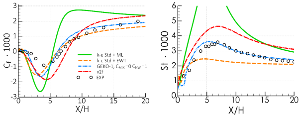
non-equilibrium flows. This can be seen in Figure 12.61: Wall shear stress coefficient, Cf (left) and wall heat transfer
coefficient, St, (right) for backward-facing step flow (12). for the Vogel and
Eaton backward facing step [12]. This flow provides experimental
data for the wall shear stress coefficient,
based models and are therefore much more flexible and accurate especially for
non-equilibrium flows. This can be seen in Figure 12.61: Wall shear stress coefficient, Cf (left) and wall heat transfer
coefficient, St, (right) for backward-facing step flow (12). for the Vogel and
Eaton backward facing step [12]. This flow provides experimental
data for the wall shear stress coefficient,  , and the heat transfer coefficient,
  , on the wall downstream of the step. The mesh for this study had a fine near
wall resolution of
, on the wall downstream of the step. The mesh for this study had a fine near
wall resolution of  .
.
Figure 12.61: Wall shear stress coefficient, Cf (left) and wall heat transfer
coefficient, St, (right) for backward-facing step flow (12). shows a model comparison for this flow. All model variants
shown are based on the same standard  model. The
  ML model is a representative of a
  low-Re model and inhibits the known
  model deficiency of substantial over-prediction of
  and
and  near the reattachment point [5]. The same
 model combined with the 2-Layer based Enhanced Wall Treatment (EWT) shows an
entirely different behavior, with a very flat distribution of the heat transfer coefficient
(but a better match of
model combined with the 2-Layer based Enhanced Wall Treatment (EWT) shows an
entirely different behavior, with a very flat distribution of the heat transfer coefficient
(but a better match of  ). The
  model in combination with the V2F approach [13]
gives an over-prediction of the separation bubble size and an overly high heat transfer
coefficient distribution. The V2F model is only included for comparison and is not offered in
any of the Ansys CFD codes. The based GEKO model with
model in combination with the V2F approach [13]
gives an over-prediction of the separation bubble size and an overly high heat transfer
coefficient distribution. The V2F model is only included for comparison and is not offered in
any of the Ansys CFD codes. The based GEKO model with  (short GEKO-1.0) model shows the best agreement of both
  and
and  . The GEKO-1.0 model is an exact transformation of the
  to a
to a  formulation, except for the sublayer model. Note that other
  models like BSL/SST models produce very similar results to GEKO. This example
shows the superior behavior of the
models like BSL/SST models produce very similar results to GEKO. This example
shows the superior behavior of the  -equation based turbulence model for predicting wall shear-stress and heat
transfer distributions compared to other approaches.
-equation based turbulence model for predicting wall shear-stress and heat
transfer distributions compared to other approaches.
Figure 12.61: Wall shear stress coefficient, Cf (left) and wall heat transfer coefficient, St, (right) for backward-facing step flow (12).
Turbulence models from the  family offer additional benefits when predicting adverse pressure gradient
flows and separation onset as will be shown in Adverse Pressure Gradients and Flow Separation.
Finally,
family offer additional benefits when predicting adverse pressure gradient
flows and separation onset as will be shown in Adverse Pressure Gradients and Flow Separation.
Finally,  models are compatible with models for laminar-turbulent transition and rough
wall treatments. All
models are compatible with models for laminar-turbulent transition and rough
wall treatments. All  models in Ansys CFD are implemented with a
  -insensitive wall treatment, avoiding the discussion concerning the optimal
selection of wall formulations in
-insensitive wall treatment, avoiding the discussion concerning the optimal
selection of wall formulations in  models (see e.g. Near-Wall Treatment). It is important
to note that the grid resolution requirements between
models (see e.g. Near-Wall Treatment). It is important
to note that the grid resolution requirements between  and
and  models are the same. In case of coarse grids (large
  ) the
) the  -insensitive wall treatment will switch automatically to a wall function
– so that there is no advantage in explicitly selecting a wall function (a choice
required in some
-insensitive wall treatment will switch automatically to a wall function
– so that there is no advantage in explicitly selecting a wall function (a choice
required in some  models).
It should be noted that there can always be cases where one turbulence model happens to be
more robust than another. In case of robustness problems with models from the  model family, it can be a prudent strategy to switch to a
  model.
Standard k- Model [14]
Use for cases where backwards compatibility is required to compare to previous simulations using this model.
Be aware that for this model no limiter (see Limiters) is activated so that excessive turbulence production can affect the simulations. Note that the lack of a limiter can lead to improved convergence (for the wrong reasons).
It is recommended to activate the 'Production Limiter'.
Note that the GEKO model with
 and
and  (an example is shown in NASA CS0 Diffuser for the
model comparison) is an exact transformation of the standard.
(an example is shown in NASA CS0 Diffuser for the
model comparison) is an exact transformation of the standard.  model – albeit with a superior wall treatment and an automatically
activated realizability limiter.
model – albeit with a superior wall treatment and an automatically
activated realizability limiter. On coarse meshes, use scalable wall functions, for finer meshes use the EWT based on the 2-layer formulation.
Realizable k- Model (RKE) [15]
Use cases where backwards compatibility is required to compare to previous simulations using this model.
Be aware that the Realizability limiter of this model is only partially effective – it allows for large turbulence production in non-shear regions (see Buoyancy Flows). The model can be combined with the 'Production Limiter'.
On coarse meshes, use scalable wall functions, for finer meshes use the EWT based on the 2-layer formulation (Near-Wall Treatment).
RNG  Model (RNGKE) [16]
Use for cases where backwards compatibility is required to compare to previous simulations using this model.
Standard  Model [7]
Do not use the standard
 model – it has a strong dependency of the solution on freestream
values of
model – it has a strong dependency of the solution on freestream
values of  outside of shear layers (see Figure 12.161: Effect of freestream omega-levels on velocity profile for free mixing layer solution.
Left: std. k-omega model without CD term. Right: GEKO model including CD term.). The model
is available mostly for historic reasons.
outside of shear layers (see Figure 12.161: Effect of freestream omega-levels on velocity profile for free mixing layer solution.
Left: std. k-omega model without CD term. Right: GEKO model including CD term.). The model
is available mostly for historic reasons.
BSL/SST Model [17], [18]
The SST model is recommended for most industrial applications. It has a high accuracy for flows with adverse pressure gradients and separation. Outside the boundary layer it reverts back to a
 model setting.
 The SST model's ability to accurately predict separation is based on the SST-limiter (Equation 12–68) which reduces the eddy-viscosity in such flows. Larger separation zones can lead to unsteady behavior, which might be physically correct, but undesirable from a project standpoint. In such cases the
 coefficient (default
  = 0.31) can be increased to values in the range of
  = 0.31-1.0 to reduce separation. Note that the
  coefficient cannot be reduced below its default value of
  = 0.31 without violating the basic calibration of the model for boundary
layers.
= 0.31 without violating the basic calibration of the model for boundary
layers.Alternatively, one can switch to the BSL model, which de-activates the SST limiter entirely.
BSL and SST models automatically activate the 'Production Limiter'.
BSL and SST models automatically activate
 -insensitive wall-treatment.
Do not use the 'low-Reynolds number correction' with any of the
 models. It is a historic feature. It is not required to integrate the
equations to the wall but can lead to pseudo-transition – meaning a non-calibrated
laminar-turbulent transition effect.
models. It is a historic feature. It is not required to integrate the
equations to the wall but can lead to pseudo-transition – meaning a non-calibrated
laminar-turbulent transition effect.
GEKO Model [10]
The model is intended to replace eventually all other two-equation models.
The model can and should be used for all industrial applications.
The model has the flexibility to allow users to tune the model against experimental data.
The model has a realizability limiter automatically activated.
The model activates the
 -insensitive wall-treatment.
The model can be tuned to mimic existing model like std.
 or SST.
 The SST is mimicked by default settings. Note that this does not mean an exact transformation of SST to GEKO.
The
 model is recovered for
  ,
,  . (An example is shown in NASA CS0 Diffuser for the
model comparison)
. (An example is shown in NASA CS0 Diffuser for the
model comparison)
The GEKO model has an adjoint formulation in Ansys Fluent which can be used as a basis for machine learning.
Note that the GEKO model is not fully published – this could lead to issues in case users want to publish their results in a scientific journal.
There is an extensive Best Practice Guide for this model available: [Generalized k-omega Two-Equation Turbulence Model (GEKO) in Ansys CFD].
The WJ-EARSM [19] can be used in case secondary flows are of importance (an example of the corner flows is shown is Corner Flows). Note however, that similar effects can be achieved by activating the simpler Corner Flow Correction (CFC) available with GEKO (and in Ansys Fluent with all other
 models) [20].
Use in combination with BSL (WJ-BSL-EARSM ) or better with GEKO model (a
 feature in Fluent .
EARSM models will not provide the same sensitivity to streamline curvature and system rotation as full RSM and additional curvature correction terms might need to be added.
These models are prone to numerical problems on complex applications and non-optimal grids. They are therefore only recommended for applications, where they have shown superior performance over eddy-viscosity models.
Examples of such applications are flows with strong curvature and or system rotation. Note however, that similar effects can be achieved when activating the Curvature Correction model in eddy-viscosity models.
In case RSM are used, it is recommended to combine them with the
 -equation (BSL or GEKO). The GEKO-RSM model formulation is based on the
stress-omega model [7]. The model solves the Reynolds stress equations in combination with
the
-equation (BSL or GEKO). The GEKO-RSM model formulation is based on the
stress-omega model [7]. The model solves the Reynolds stress equations in combination with
the  -equation from the GEKO model instead of the original Wilcox model.
The eddy-viscosity assumption alters the production term,  , in the
  -equation from a term linear in the velocity gradients to a quadratic term
(
-equation from a term linear in the velocity gradients to a quadratic term
( ). This can cause problems in regions with non-shear layer related strain
rate,
). This can cause problems in regions with non-shear layer related strain
rate,  , like in inviscid stagnation or in acceleration zones. When using
two-equation eddy-viscosity models, limiters must therefore be employed. Limiters are not
required when running the WJ-EARSM as it restricts the level of production over dissipation
automatically. Examples for the use of limiters are given in Limiters.
, like in inviscid stagnation or in acceleration zones. When using
two-equation eddy-viscosity models, limiters must therefore be employed. Limiters are not
required when running the WJ-EARSM as it restricts the level of production over dissipation
automatically. Examples for the use of limiters are given in Limiters.
For  models, the user needs to activate a limiter. For the std.
  model no limiter is active by default (representing the published version of
the model) and the production limiter should be activated. For the RKE model a realizability
limiter is built-in, but experience shows that it does not work effectively, due to the
specifics of its formulation. Also, for this model the production limiter is recommended. Note
that when writing a report/publication the activation of limiters should be clearly indicated
to allow a proper interpretation and reproduction of the results.
model no limiter is active by default (representing the published version of
the model) and the production limiter should be activated. For the RKE model a realizability
limiter is built-in, but experience shows that it does not work effectively, due to the
specifics of its formulation. Also, for this model the production limiter is recommended. Note
that when writing a report/publication the activation of limiters should be clearly indicated
to allow a proper interpretation and reproduction of the results.
All  -equation based models in Ansys Fluent and Ansys CFX have the production limiter
automatically activated. The GEKO model features in addition a proper realizability limiter.
-equation based models in Ansys Fluent and Ansys CFX have the production limiter
automatically activated. The GEKO model features in addition a proper realizability limiter.
When models for laminar-turbulent transition are activated, it was found that in some cases the production limiter was not sufficient to prevent a minor build-up of turbulence in the stagnation zone of airfoils. This is usually unnoticeable in fully turbulent mode but can slightly affect the transition location. For this reason, the Kato-Launder limiter [21] is additionally activated for such flows. This limiter can affect other parts of the flow, especially flows with swirl and curvature. In case this is not acceptable, this limiter can be deactivated.
For
 models, activate the production limiter manually.
For
 models no action is required.
For transition models – no action is required unless the Kato-Launder limiter is not wanted.
The following sections describe model additions which can be used in combination with two-equation models. Particularly, Corner Correction [20] and Curvature Corrections [22], [23] are meant to eliminate some deficiencies of eddy-viscosity models relative to fully Reynolds-Stress Models. Other additions, like rough walls and laminar-turbulent transition are required for all RANS models if the effects are important for the intended application.
The following topics are discussed:
There are four models for laminar-turbulent transition in Ansys Fluent and Ansys CFX:
The algebraic intermittency model (Ansys Fluent)
The One-equation intermittency model (Ansys Fluent, Ansys CFX)
The two equation
 model (Ansys Fluent, Ansys CFX)
 Model (Ansys Fluent)
The first three models are based on the concept of 'Local-Correlation based Transition
Modeling – LCTM'. They form a series of models as developed over time starting with the
 model [24]–[26] which was then simplified to a one-equation model and finally to an algebraic model. The
models are calibrated in a similar fashion, but offer differences in their predictions. Users
are therefore advised to test which model best suits their test cases. Obviously, the CPU cost
increases with the number of transport equations being solved. The algebraic model might
therefore serve as a good starting point. The
model [24]–[26] which was then simplified to a one-equation model and finally to an algebraic model. The
models are calibrated in a similar fashion, but offer differences in their predictions. Users
are therefore advised to test which model best suits their test cases. Obviously, the CPU cost
increases with the number of transport equations being solved. The algebraic model might
therefore serve as a good starting point. The  formulation models the kinetic energy in the pre-transitional phase of the
boundary layer and triggers transition based on this quantity. It is not widely used and not
recommended, as it is only compatible with the standard
formulation models the kinetic energy in the pre-transitional phase of the
boundary layer and triggers transition based on this quantity. It is not widely used and not
recommended, as it is only compatible with the standard  model.
Including the effect of transition into the CFD simulation requires finer mesh resolution (see Transitional Boundary Layers) and should therefore be employed with caution.
Transition prediction is important for aerodynamic and turbomachinery flows, as transition can strongly affect overall performance. It is also important to include in some heat transfer cases like impinging jets, as laminar flows have a much lower heat transfer coefficient than turbulent flow.
In case transition is important, it has strong implications on the set-up from a modeling, numerical and mesh resolution standpoint.
Select a suitable transition model
The mesh resolution requirements for predicting transition are much higher than for fully turbulent flow simulations. This is discussed in Transitional Boundary Layers.
Numerical settings might need to be adjusted.
Monitor points/charts on transition location motion should be included to check convergence. Plotting charts of wall shear stress of
 during iterations is recommended to visually see if the transition
locations are settling down.
during iterations is recommended to visually see if the transition
locations are settling down.
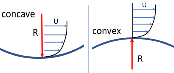
Streamline curvature and swirl can have a significant effect on turbulence. This is illustrated in Figure 12.62: Schematic of the boundary layer on curved surfaces. which shows on the left a boundary layer on a concave wall and on the right a boundary layer on a convex wall. In the concave case, turbulence is enhanced and for the convex case it is damped. Standard eddy-viscosity models do not account for this effect and need augmentation to sensitize them. The effect of curvature is even stronger for swirling flows, where turbulence is typically strongly suppressed (see Swirl Flows).
The Curvature Correction [22] used in Ansys-CFD is based on
the so-called Spalart-Shur correction [23]. The details of the
formulation can be found in the theory documentation and are not reported here. This correction
detects changes in streamline direction due to changes in the orientation of the strain rate
tensor along a streamline. This then results in a correction factor which multiplies the
production terms of both the  - and the
  -equations. For stabilizing curvature, the factor is smaller and for
de-stabilizing flows larger than one.
-equations. For stabilizing curvature, the factor is smaller and for
de-stabilizing flows larger than one.
The CC is most relevant not for boundary layers but for free vortex flows, where the effect of curvature results in strong damping of turbulence inside the vortex. Models without CC provisions produce much too high eddy-viscosities in such scenarios and strongly damp the vortex.
Turbulence can be dampened or enhanced based on streamline curvature (see Swirl Flows). The Correction should be activated if curvature effects are strong and important. This is typically the case if the radius of curvature is of the same order or smaller than the boundary/shear-layer thickness. Note that for most boundary layer flows this is not the case.
This correction is most beneficial for swirling flows (tip vortex of a wing, vortex inside a hydro-cyclone). Eddy-viscosity models without this correction create excessive eddy-viscosity levels in such flows and reduce vortex strength too strongly. In addition, they enforce a solid body-like rotation, whereas a real vortex often has significant regions following inviscid laws.
In principle, the correction does not hurt flows without or with only weak curvature but increases computational costs.
Another physical effect which cannot be represented by eddy-viscosity models is the secondary flow caused by turbulence through anisotropy of the normal stresses (meaning that the normal stresses in the wall parallel and wall normal directions are different, driving a secondary flow). This effect appears typically in corner flows (like rectangular channels). One strategy to enable eddy-viscosity models to account for this effect is to extend them through a non-linear stress-strain relationship (see EARSM models in Corner Flows). The simplest formulation is however the Quadratic Closure Relation (QCR) proposed by Spalart [20]. It consists of extending the linear part of the eddy-viscosity formulation by a quadratic term:
 | (12–38) |
with

The effect is important for:
Flows parallel to corners, like those observed in wing-body junctions or rectangular channels, which develop secondary flow directed into the corner. This effect (Prandtl's secondary flows of 2nd kind, 27) cannot be captured by eddy-viscosity models, as the effect is driven by the anisotropy of the normal stresses of the Reynolds Stress tensor.
Without this correction, the flow in such corners can show premature separation if encountering an adverse pressure gradient. This can have a significant effect on the overall flow and can potentially lead to incorrect flow topologies in the CFD simulation. The resulting errors can be very large, as a change in flow topology (e.g. separation from a corner instead from the clean part of the wing/blade) can affect most other flow parameters.
Simulations will only benefit from this correction if there is a sufficiently fine grid resolution in the corner region. Hexahedral meshes are optimal for such flows, as they allow for an easy adaptation of the surface grid lines into the corner.
This correction should not produce negative side-effects in terms of accuracy if activated in cases where it is not required. However, it can potentially affect robustness and CPU cost.
Flows with gradients in density in a gravity field can exhibit similar effects as flows
with curvature. Flows where the force vector due to gravity and the density gradient point in
the same direction are stabilized (decrease in turbulence) whereas the opposite is true for
flows where the two vectors point in opposite directions. Buoyancy terms have been developed
originally for the  model. The source term in the
  -equation reads (
 – gravity vector):
 | (12–39) |
To judge if such effects are important, this term has to be set in relation to the
production of turbulence kinetic energy. For shear layers one gets (with  ,
,  – velocity, density differences across shear layer,
  thickness of layer,
  ):
):
 | (12–40) |
In case this ratio is larger than a threshold (of the order of  > 0.1) the term
  should be included. As outlined in the theory documentation, the term can
additionally be included into the scale-equation (
should be included. As outlined in the theory documentation, the term can
additionally be included into the scale-equation ( /
/ -equation). Since the benefit of doing so is not consistent, the default is to
include the term only into the
-equation). Since the benefit of doing so is not consistent, the default is to
include the term only into the  -equation.
The effect of buoyancy is similar to the effect of curvature – it can stabilize or destabilize turbulence.
Turbulence is enhanced/damped if the density gradient and gravity vector point in opposite/same directions.
Rough walls can have a significant effect on the performance of technical devices. Roughness has two essential effects. The first is that it increases wall shear stress levels (and thereby also heat transfer) and the second is that it forces laminar-turbulent transition to more upstream locations.
There are several roughness options in Ansys CFD:
The standard method is a simple shift of the logarithmic layer based on wall roughness. In addition, the cell center of the wall cell is virtually shifted as:
 where
where  is the roughness height. This option is used in Ansys Fluent.
 The second method is a blend of the Wilcox wall roughness model [7] and the log-layer shift, based on
 . This option is the default for all
  -equation based models in Ansys CFX.
The last option is proposed by Aupoix [28] and modifies the near wall boundary values of the turbulence quantities to achieve the desired increase in wall-shear. It can be applied to the Spalart-Allmaras model and all
 -based two-equation models.
The first two options are compatible with all  values if
  lies in the inner region (~0.1 of the boundary layer thickness).
The Aupoix formulation requires a fine near wall mesh ( ~1) but can cover roughness heights which are a significant fraction of the
boundary layer height.
~1) but can cover roughness heights which are a significant fraction of the
boundary layer height.
Roughness effects on transition location can also be included into the SST  transition model (4-equation model). The effect of roughness is to push the
transition location upstream. While the effect of fully turbulent flow is described by the
sand-grain roughness, the effect on transition is determined by the height of the roughness
elements (geometric roughness), as even a single roughness element can trigger transition.
transition model (4-equation model). The effect of roughness is to push the
transition location upstream. While the effect of fully turbulent flow is described by the
sand-grain roughness, the effect on transition is determined by the height of the roughness
elements (geometric roughness), as even a single roughness element can trigger transition.