


The following topics are discussed:
For a detailed discussion of the derivation of turbulence equations please consult one of the available text books ([2]–[7]). In this section only a very basic model descriptions will be provided to allow the connection between the best Practice discussions and the turbulence model formulations.
The following topics are discussed:
Due to the high cost of DNS, the engineering approach to CFD lies in the Reynolds-Averaged Navier-Stokes (RANS) equations. These equations are obtained from the exact Navier-Stokes equations through time (or ensemble) averaging.
Time averaging is defined by:
 | (12–42) |
 | (12–43) |
In other words, the instantaneous quantity  is split into a time-mean value
  and a fluctuating part
  . The simulation is then only concerned with the time-mean
part. More generally, one can also perform an ensemble-averaging over many instances of an
experiment:
. The simulation is then only concerned with the time-mean
part. More generally, one can also perform an ensemble-averaging over many instances of an
experiment:
Ensemble averaging is defined by:
 | (12–44) |
 | (12–45) |
The advantage of ensemble averaging is that it can also be applied to inherently unsteady flows (e.g. the flow in an internal combustion engine with moving parts). Both forms of averaging lead to the same equations and turbulence models, so the same overbar is used for simplicity.
When these averaging processes are applied to the Navier-Stokes equations, one obtains the RANS momentum equations:
 | (12–46) |
where ( ) ?is the vector of the averaged velocity field,
  is the density (assumed
constant in this brief overview),
is the density (assumed
constant in this brief overview),  is the averaged pressure and
  is the Stokes (laminar)
stress tensor. For incompressible flows:
is the Stokes (laminar)
stress tensor. For incompressible flows:
 | (12–47) |
with  being the dynamic molecular viscosity.
The last term in the above equation ( ) is so-called 'Reynolds Stress
Tensor' and results from the averaging of the non-linear convection terms. This tensor
represents the influence of the turbulent fluctuations on the mean velocity field. The above
momentum equations are 'unclosed' as no equations are yet available for the Reynolds Stress
Tensor. Turbulence models are needed to provide formulations for this tensor.
) is so-called 'Reynolds Stress
Tensor' and results from the averaging of the non-linear convection terms. This tensor
represents the influence of the turbulent fluctuations on the mean velocity field. The above
momentum equations are 'unclosed' as no equations are yet available for the Reynolds Stress
Tensor. Turbulence models are needed to provide formulations for this tensor.
The RANS momentum equations above are derived under the assumption that there are no significant density variations due to turbulence – this is typically the case for flows with Mach numbers below 3. Note that density variations on the mean flow occur much earlier, starting as low as M~0.1.
The most widely applied assumption in turbulence modeling is the eddy-viscosity assumption. It is based on the concept that turbulent stresses can be represented in a similar fashion as the laminar stress tensor:
 | (12–48) |
The last term on the right represents the turbulent kinetic energy,  , and accounts for
the requirement that the sum of the diagonals of the Reynolds Stress Tensor must amount to
, and accounts for
the requirement that the sum of the diagonals of the Reynolds Stress Tensor must amount to  .
This term is not essential and can be avoided/ignored (e.g. in one-equation models where
.
This term is not essential and can be avoided/ignored (e.g. in one-equation models where  is
not available)
is
not available)
The original problem of providing closure equations for the six (due to symmetry of
tensor) unknowns of the Reynolds Stress Tensor is thereby now reduced to providing a suitable
eddy-viscosity  (also called turbulent viscosity). It is important to note that
  is not a
property of the fluid, but a property of the local turbulence. The eddy-viscosity has
dimension:
is not a
property of the fluid, but a property of the local turbulence. The eddy-viscosity has
dimension:
 | (12–49) |
where  and
and  are the length- and time-scales of turbulence, respectively.
Contrary to the eddy-viscosity assumption, there are methods, which aim at computing the individual Reynolds Stresses individually. For this purpose, exact transport equations for each Reynolds Stress are derived (6 equations). These exact equations, however, contain again new unknown terms which need to be modeled (see e.g. [5]). Different modeling assumptions for these terms then leads to a large variety of Reynolds Stress Models (RSM). The exact RSM equations read:
 | (12–50) |
The terms in these equations are: Line 1: time derivative, convection, production. Line
2: pressure strain (PS), dissipation. Line 3: turbulent diffusion and molecular diffusion. All
terms in Line 1 are exact and need no modeling. This is true also for the last term in Line 3.
All other terms require models to close the equations. In addition, there is a need for
information on the turbulent scale required e.g. in the dissipation term. This information is
typically obtained from an additional transport equation (e.g.  -equation of
  -equation). All
in all, RSM closure therefore requires the solution of seven additional equations. Proposed RSM
differ mostly by the way they model the pressure-strain term.
-equation). All
in all, RSM closure therefore requires the solution of seven additional equations. Proposed RSM
differ mostly by the way they model the pressure-strain term.
Simplified versions of RSM models can be obtained where the Reynolds stresses are computed from algebraic formulations instead of transport equations. Such models are generically of the form:
 | (12–51) |
with
 | (12–52) |
and  being the turbulent kinetic energy and
  a turbulent frequency scale. Note that the
eddy-viscosity formulation (Eq. (9.7)) is the simplest form of such a model. The main model in
Ansys CFD is the version of Wallin-Johansson (19).
a turbulent frequency scale. Note that the
eddy-viscosity formulation (Eq. (9.7)) is the simplest form of such a model. The main model in
Ansys CFD is the version of Wallin-Johansson (19).
All industrial relevant two-equation models use the equation for the turbulent kinetic
energy,  , to provide one of the two scales required. The
  -equation can be derived by summing
up half of the diagonal of the exact RSM equations (Eq.(9.9)).
-equation can be derived by summing
up half of the diagonal of the exact RSM equations (Eq.(9.9)).
 | (12–53) |
with:
 | (12–54) |
 | (12–55) |
 | (12–56) |
The term  is the production term. When inserting the eddy-viscosity formulation (Equation
(9.7)) it can be formulated as:
is the production term. When inserting the eddy-viscosity formulation (Equation
(9.7)) it can be formulated as:
 | (12–57) |
with 
The term  is the turbulence energy dissipation rate, which converts turbulent kinetic energy into heat
(typically small enough to be neglected in the overall energy balance).
is the turbulence energy dissipation rate, which converts turbulent kinetic energy into heat
(typically small enough to be neglected in the overall energy balance).
The term  is called turbulent diffusion. In an integral sense, it does not contribute to
the overall production or dissipation of turbulent kinetic energy, but does only smooths out
the
is called turbulent diffusion. In an integral sense, it does not contribute to
the overall production or dissipation of turbulent kinetic energy, but does only smooths out
the  -distribution. It is typically modeled by a simple gradient-diffusion hypothesis:
 | (12–58) |
The modeled  -equation therefore reads:
 | (12–59) |
With these formulations, the only term missing (unclosed) in the  -equation is the
dissipation term
-equation is the
dissipation term  . It needs to be provided from a separate scale-equation (e.g. the
  -equation
or the
-equation
or the  -equation with
  ).
).
What is meant by 'turbulent scales' in the context of RANS modeling? As discussed in the introduction, turbulence consists of a spectrum of scales – so identifying a single length- or time-scale is not trivial. However, the mixing processes which are of foremost engineering interest are driven by the largest scales of turbulence.
The derivation of the scale equation (typically  or
or  ) is one of the weakest steps in
RANS modeling. While exact transport equations can be derived e.g. for
) is one of the weakest steps in
RANS modeling. While exact transport equations can be derived e.g. for  , such equations
represent the small scales of turbulence (where dissipation takes place) and do not provide
information on the large scales required in RANS closure. One could argue that in RANS
, such equations
represent the small scales of turbulence (where dissipation takes place) and do not provide
information on the large scales required in RANS closure. One could argue that in RANS  is not
trying to model 'dissipation' but rather the destruction of large scales into smaller scales
– which are no longer relevant for the mixing processes.
is not
trying to model 'dissipation' but rather the destruction of large scales into smaller scales
– which are no longer relevant for the mixing processes.
To arrive at a suitable model equation, the assumption is made that the scale equation has
a form similar to the  -equation:
 | (12–60) |
with the ratio  introduced for dimensional correctness. The coefficients
  ,
, ,
,  are model coefficients which need to be tuned by experimental data. The coefficients of the
standard
are model coefficients which need to be tuned by experimental data. The coefficients of the
standard  model are:


An equation for the turbulent frequency,  can be derived with the same arguments:
 | (12–61) |
With this set of equations, the eddy-viscosity can be computed:
 | (12–62) |
using 


Since  and
and  are related, one can investigate the differences between the
  and the
 equations. This can be achieved e.g. by transforming the exact
  equation to an
  equation.
Assuming for simplicity
equation.
Assuming for simplicity  one gets:
 | (12–63) |
With the cross-diffusion term:
 | (12–64) |
The transformation of the coefficients gives the relation:
 | (12–65) |
In other words, the  -equation when derived on the same dimensional arguments as the
 -equation results in Equation ((9.20), whereas the transformation of the
  -equation into a
 -equation gives Equation (9.22). The difference lies mainly in the cross-diffusion term
  .
.
What is the effect of the  term? There are two main effects, one positive and one negative. The negative
effect is discussed in detail by Wilcox [7] and is manifested in an improved performance of the
term? There are two main effects, one positive and one negative. The negative
effect is discussed in detail by Wilcox [7] and is manifested in an improved performance of the  -equation based models not utilizing the
  term in adverse pressure gradient boundary layers. Such models predict an
improved response to the pressure gradient and a higher sensitivity to predict flow separation,
compared to
term in adverse pressure gradient boundary layers. Such models predict an
improved response to the pressure gradient and a higher sensitivity to predict flow separation,
compared to  -equation based models. In other words, the inclusion of the
  term in the
  -equation in the near wall region would inhibit correct
separation prediction.
-equation in the near wall region would inhibit correct
separation prediction.
The second effect of including the  is desirable, as it avoids the strong sensitivity of the standard
 -equation (models without
  ) based model to freestream values. As discussed in detail in [52] the
standard model produces a wide variation in results in case the level of
) based model to freestream values. As discussed in detail in [52] the
standard model produces a wide variation in results in case the level of  changes outside the boundary or free shear layer (freestream). This is
illustrated in Figure 12.161: Effect of freestream omega-levels on velocity profile for free mixing layer solution.
Left: std. k-omega model without CD term. Right: GEKO model including CD term. for a mixing layer. The left part of the
Figures shows the reaction of the Wilcox
changes outside the boundary or free shear layer (freestream). This is
illustrated in Figure 12.161: Effect of freestream omega-levels on velocity profile for free mixing layer solution.
Left: std. k-omega model without CD term. Right: GEKO model including CD term. for a mixing layer. The left part of the
Figures shows the reaction of the Wilcox  model to changes in freestream
  on the velocity profile and the right part shows the same test using the GEKO
 model (which includes the
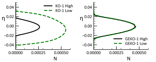
  term). Figure 12.162: Effect of freestream
  -levels on non-dimensional eddy viscosity profiles for free mixing layer solution. Left: standard
  model without CD term. Right: GEKO model including CD term. shows the same effect on the
eddy-viscosity profiles, where the difference in the standard
model without CD term. Right: GEKO model including CD term. shows the same effect on the
eddy-viscosity profiles, where the difference in the standard  model is more than a factor 2 between the low and the high freestream values.
Since the level of freestream values cannot easily be controlled and is often based on roughly
estimated inlet values, solution independence from these values is essential for reliable
simulations.
model is more than a factor 2 between the low and the high freestream values.
Since the level of freestream values cannot easily be controlled and is often based on roughly
estimated inlet values, solution independence from these values is essential for reliable
simulations.
Figure 12.161: Effect of freestream omega-levels on velocity profile for free mixing layer solution. Left: std. k-omega model without CD term. Right: GEKO model including CD term.
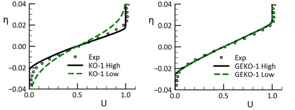
Figure 12.162: Effect of freestream -levels on non-dimensional eddy viscosity profiles for free mixing layer solution. Left: standard model without CD term. Right: GEKO model including CD term.
The equations discussed so far form the basis of all industrially  and
and  based
turbulence models.
based
turbulence models.
The motivation behind two-equation models originates from the need to obtain the two scales
required to compute the eddy-viscosity. Based on dimensional arguments, a length-scale, , and
a time-scale,
, and
a time-scale,  , are required for that purpose. Note that any two other scales are equivalent
as there are only two independent mechanical scales. These requirements naturally lead to
two-equation models as a basis for providing these scales. However, two-equation models also
form the basis for all further developments, like One-equation models, Reynolds Stress Models
(RSM) or Explicit Algebraic Reynolds Stress models (EARSM). Two-equation models are also the
optimal platform for including additional physics, like laminar-turbulent transition, rough
walls, buoyancy, as well as hybrid RANS-LES concepts.
, are required for that purpose. Note that any two other scales are equivalent
as there are only two independent mechanical scales. These requirements naturally lead to
two-equation models as a basis for providing these scales. However, two-equation models also
form the basis for all further developments, like One-equation models, Reynolds Stress Models
(RSM) or Explicit Algebraic Reynolds Stress models (EARSM). Two-equation models are also the
optimal platform for including additional physics, like laminar-turbulent transition, rough
walls, buoyancy, as well as hybrid RANS-LES concepts.
Two-equation models are composed of the following elements:
Turbulent kinetic energy equation
Scale equation (
 or
or  )
)Eddy-viscosity formulation
Near-wall treatment
Limiters
Each one of these elements can have a substantial influence of accuracy and robustness of the simulations.
The following topics are discussed:

The BSL/SST Models
Based on the investigation of the freestream dependency of the Wilcox model [52], Menter
proposed model formulations which are composed of a blend of  and
and  model elements (17).
As discussed in Section 9.2.2, the main difference between these models is the cross-diffusion
term (CD) which appears when transforming the
model elements (17).
As discussed in Section 9.2.2, the main difference between these models is the cross-diffusion
term (CD) which appears when transforming the  model to a
  model. This term avoids the
freestream sensitivity near the shear/boundary layer edge. However, while it is desirable to
include the term near the shear/boundary layer edge, it is not desirable to activate it near
the wall, as it negatively affects the adverse pressure gradient behavior of the model. The BSL
model was therefore built on the blending function
model. This term avoids the
freestream sensitivity near the shear/boundary layer edge. However, while it is desirable to
include the term near the shear/boundary layer edge, it is not desirable to activate it near
the wall, as it negatively affects the adverse pressure gradient behavior of the model. The BSL
model was therefore built on the blending function  , which is based on wall distance,
  . The
function has a value of
. The
function has a value of  inside the wall boundary layer and gradually blends to
  in the
outer part of the boundary layer and beyond. This function blends the
in the
outer part of the boundary layer and beyond. This function blends the  term into the
 -equation but also blends the coefficients from those of the
  to those of the
  model.
 | (12–66) |
 | (12–67) |
 | (12–68) |
 | (12–69) |
 | (12–70) |


There are two model variants. The BSL (baseline model) and the SST (Shear Stress
Transport) model. The SST model is based on the BSL model, but in addition limits the
eddy-viscosity inside the boundary layer (using a second blending function  ) to achieve
improved model performance for flows under adverse pressure gradients and separation.
) to achieve
improved model performance for flows under adverse pressure gradients and separation.
The two blending functions  and
and  read:
read:
 | (12–71) |
 | (12–72) |
The BSL model can also be used as the basis for combination with EARSM and RSM models - where the limiter on the eddy-viscosity is not required, as improved stress prediction is achieved through the EARSM/RSM formulation. The SST model on the other hand is calibrated for accurate prediction of separation and aerodynamic flows when used as an eddy-viscosity model.
There is a clear increase in complexity from the Wilcox model to the BSL/SST models, mainly through the need for blending functions, which in turn require the wall-distance. Wall-distance is not problematic if the mesh/geometry are fixed (as is the case in most CFD simulations). In case of varying mesh/geometry however, the wall distance computation can become expensive as it needs to be repeated for every time-step. Particularly for massively parallel simulations, the wall distance computation can dominate the CPU costs as the algebraic operation does not scale well on such machines. The GEKO model (Section 3.3.2) has therefore been developed with an option avoiding the wall distance.
The SST model allows variation of the  coefficient without affecting the calibration of
the logarithmic layer. Its value can be increased, thereby reducing the sensitivity to adverse
pressure gradient flows and delaying/reducing flow separation. The value cannot be decreased
however, as that would interfere with the log-law behavior and would thereby negatively affect
the flat plat calibration.
coefficient without affecting the calibration of
the logarithmic layer. Its value can be increased, thereby reducing the sensitivity to adverse
pressure gradient flows and delaying/reducing flow separation. The value cannot be decreased
however, as that would interfere with the log-law behavior and would thereby negatively affect
the flat plat calibration.
The Generalized  model (GEKO)
The main characteristics of the GEKO model is that it has several free parameters for tuning the model to different flow scenarios. The starting point for the formulation is:
 | (12–73) |
 | (12–74) |
 | (12–75) |
 | (12–76) |
 | (12–77) |
 | (12–78) |
There is a provision for corner flows which amounts to adding a quadratic term to the stress-strain relation. The terms is essentially the same as the Quadratic Closure Relation (QCR) proposed by Spalart [53]:
 | (12–79) |
The GEKO model formulation is otherwise conventional, it involves the cross-diffusion term
which typically is derived from a transformation of the  model to a
  . This term is
included in most of the more recent
. This term is
included in most of the more recent  models in various ways. It is generally understood that
this term is required at the edge of turbulent layers to maintain the
models in various ways. It is generally understood that
this term is required at the edge of turbulent layers to maintain the  model behavior and
avoid freestream sensitivities.
model behavior and
avoid freestream sensitivities.
The main difference of GEKO to existing models is the introduction of free parameters which can be tuned by the user to achieve different goals in different parts of the simulation domain. The details of the GEKO model formulation are not published at this point, but the effect of the free parameters will be described. Note that an entire 'Best Practice Guide' exists for the GEKO model: [1].
Currently there are the following parameters included for tuning:
 – Parameter to optimize flow separation from smooth surfaces
 – Parameter to optimize flow in non-equilibrium near wall regions
(heat transfer,
– Parameter to optimize flow in non-equilibrium near wall regions
(heat transfer,  , ….)
, ….) – Parameter to optimize strength of mixing in free shear flows
 – Parameter to optimize free shear layer mixing (optimize free jets
independent of mixing layer)
– Parameter to optimize free shear layer mixing (optimize free jets
independent of mixing layer) – Parameter to optimize flows with streamline curvature and rotation
 – Parameter to optimize anisotropic flow in corners
All these parameters are designed so that they do not negatively affect the basic model
calibration for flat plate flows. In other words, the logarithmic layer formulation is
preserved despite the changes in these parameters. Note that the two last parameters can also
be combined with other  models.
All parameters (except  ) are available through User Defined Functions (UDF) access.
This means that they can be defined either with a global value (in the GUI/TUI) or as
zonal/local values via UDFs.
) are available through User Defined Functions (UDF) access.
This means that they can be defined either with a global value (in the GUI/TUI) or as
zonal/local values via UDFs.
The function  is defined using the blending function
  :
:
 | (12–80) |
Inside wall boundary layers, the term is de-activated ( =1) to ensure that the
 /
/ coefficient only affects free shear flows. It is also seen, that the coefficient
  only affects the impact of
  (e.g. in case
  =0 also
  has no effect).
  essentially
reduced the impact of
essentially
reduced the impact of  on jet flows (where
  would otherwise cause an over-prediction of
jet spreading rates).
would otherwise cause an over-prediction of
jet spreading rates).
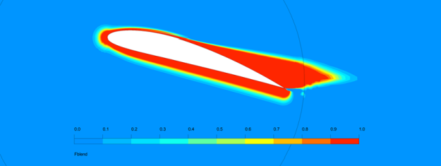
Figure 12.163: Blending function FBlend for introducing addtional mixing through coefficients  /
/ . shows the function
  for a NACA 4412 airfoil at
  =12° angle of attack. The function is
  =1 (red) inside the boundary layer and
  =0 (blue) away from the wall. Especially at the trailing edge, where the wake
(free shear flow) leaves the wall (boundary layer) the function switches swiftly to activate
the
=0 (blue) away from the wall. Especially at the trailing edge, where the wake
(free shear flow) leaves the wall (boundary layer) the function switches swiftly to activate
the  -term.
The free coefficients should be in the range:


The coefficient  can in principle be increased beyond
  =1, in cases with very
strong mixing.
=1, in cases with very
strong mixing.
The main tuning parameter for the GEKO model is the coefficient  . When increasing
 , boundary layer separation will be predicted more aggressively. However, in addition, the
spreading rates of all free shear flows will be affected by changes in
, boundary layer separation will be predicted more aggressively. However, in addition, the
spreading rates of all free shear flows will be affected by changes in  as it generally
decreases the eddy-viscosity level in the entire domain. This is not convenient for users, as
they would have to tune 2 parameters simultaneously. To maintain the spreading rate for the
most important free shear flow, namely the mixing layer, while changing
as it generally
decreases the eddy-viscosity level in the entire domain. This is not convenient for users, as
they would have to tune 2 parameters simultaneously. To maintain the spreading rate for the
most important free shear flow, namely the mixing layer, while changing  , a correlation was
developed, which maintains the mixing layer spreading rates under changes of
, a correlation was
developed, which maintains the mixing layer spreading rates under changes of  :
:
 | (12–81) |
This correlation is set as default – however users can also optimize  by hand,
independently of
by hand,
independently of  .
.
The parameter  is designed to reduce the spreading rate for round jets, which is over-predicted
with all cnventional turbulence models. To achieve optimal performance for round jets, one needs to set
is designed to reduce the spreading rate for round jets, which is over-predicted
with all cnventional turbulence models. To achieve optimal performance for round jets, one needs to set
 to values
  ~1.75-2.00 and
  =0.9 (default). With reduction in
  and the corresponding reduction in
  , the effect of
  vanishes (see [Generalized k-omega Two-Equation Turbulence Model (GEKO) in Ansys CFD ].). There is another parameter CJET_AUX which
also has an influence on the jet flow. It defines the limit between mixing layers and jet flows.
The larger the value, the sharper the 'demarcation' and stronger the effect of
vanishes (see [Generalized k-omega Two-Equation Turbulence Model (GEKO) in Ansys CFD ].). There is another parameter CJET_AUX which
also has an influence on the jet flow. It defines the limit between mixing layers and jet flows.
The larger the value, the sharper the 'demarcation' and stronger the effect of  . The default value is CJET_AUX=2.0. It is suitable for jet flow
simulations to set the CJET_AUX=4.0. This is not done by default, as it can lead to oscillations
on poor meshes. For more details and test cases, see the Best Practices Guidelines for the GEKO
model [Generalized k-omega Two-Equation Turbulence Model (GEKO) in Ansys CFD ].
. The default value is CJET_AUX=2.0. It is suitable for jet flow
simulations to set the CJET_AUX=4.0. This is not done by default, as it can lead to oscillations
on poor meshes. For more details and test cases, see the Best Practices Guidelines for the GEKO
model [Generalized k-omega Two-Equation Turbulence Model (GEKO) in Ansys CFD ].
At first, the versatility of the model seems to pose a challenge to the user as to the
optimal selection of coefficients. However, there are strong defaults and there are certain
combinations of coefficients, which can be applied to most flows, so that the user would only
interfere on specific cases, where the model does not lead to satisfactory results. The
selection of  results in an exact transformation to the
  model, albeit with
improved sub-layer treatment and limiters activated.
model, albeit with
improved sub-layer treatment and limiters activated.

The standard  -Model
In order to explain the preference for  -equation based models, it is important to
critically discuss the
-equation based models, it is important to
critically discuss the  -equation. It needs to be emphasized that the
  -equation has been used
in many CFD simulations in the past which is a clear indication that the issues discussed below
are not present in all or even the majority of
-equation has been used
in many CFD simulations in the past which is a clear indication that the issues discussed below
are not present in all or even the majority of  -equation model simulations. However, these
deficiencies are frequent enough to preclude the
-equation model simulations. However, these
deficiencies are frequent enough to preclude the  -equation as a turbulence model integration
platform.
-equation as a turbulence model integration
platform.
The standard  model without Viscous Sublayer Model (VSM) terms is given by:
 | (12–82) |
 | (12–83) |
 | (12–84) |


The  model provides a 'middle of the road' calibration which covers many flows with
sensible accuracy – which might explain its popularity over the years.
model provides a 'middle of the road' calibration which covers many flows with
sensible accuracy – which might explain its popularity over the years.
A well-published deficiency of the  -equation is the lack of response to adverse pressure
gradient flows [7], (17). The model produces too large turbulence length scales near the wall
and thereby delays or even suppresses flow separation when compared to experimental data. This
in turn leads to overly optimistic design choices as the model predicts attached flow under
conditions, where the real flow can already be severely separated.
-equation is the lack of response to adverse pressure
gradient flows [7], (17). The model produces too large turbulence length scales near the wall
and thereby delays or even suppresses flow separation when compared to experimental data. This
in turn leads to overly optimistic design choices as the model predicts attached flow under
conditions, where the real flow can already be severely separated.
This effect can be seen for a diffuser flow [54]. It consists of a straight wall on one
side and an inclined wall on the other. The flow in the experiment separates from the inclined
wall. Figure 12.164: Flow topology for Obi [54] diffuser. Top - SST model. Bottom ![Flow topology for Obi [] diffuser. Top - SST model. Bottom model.](graphics/eqf508aaca-82c7-4dc3-9da1-234abe5d6e1e.svg) model. shows the different flow topologies predicted by the
SST and the
model. shows the different flow topologies predicted by the
SST and the  model. Figure 12.165: Velocity profiles for Obi diffuser [54]. Comparison of SST,
 ![Velocity profiles for Obi diffuser []. Comparison of SST, and experimental data.](graphics/eq8bd3442e-ae88-4bb1-bd07-16a2c3c43df7.svg) and experimental data. provides a comparison of the model
predictions with the exp. velocity profiles which clearly shows that the flow is separated as
predicted by the SST model. In case where the design engineer would base the decision of the
opening angle of the diffuser on the
and experimental data. provides a comparison of the model
predictions with the exp. velocity profiles which clearly shows that the flow is separated as
predicted by the SST model. In case where the design engineer would base the decision of the
opening angle of the diffuser on the  model, the real performance (pressure loss) would be much more optimistic
than later observed when the device is built.
model, the real performance (pressure loss) would be much more optimistic
than later observed when the device is built.
![Flow topology for Obi [] diffuser. Top - SST model. Bottom model.](graphics/image273.png)
![Velocity profiles for Obi diffuser []. Comparison of SST, and experimental data.](graphics/image274.png)
It is important to emphasize that similar pictures of failure could be produced for almost
any turbulence model, as there are always flows where models struggle. However, the ability to
accurately predict separation onset is essential for many applications, and the  based
models have never been able to overcome their deficiencies in this respect.
based
models have never been able to overcome their deficiencies in this respect.
The Realizable  Model (RKE)
The RKE model is a variation of the standard  model. Its derivation is somewhat
curious, involving a mix of small and large scale arguments (15), but this is of no relevance
in the current document. The equations read:
model. Its derivation is somewhat
curious, involving a mix of small and large scale arguments (15), but this is of no relevance
in the current document. The equations read:
 | (12–85) |
 | (12–86) |
 | (12–87) |
 | (12–88) |
 | (12–89) |


One of the lesser appreciated
deficiencies of two-equation models is their behavior in inviscid regions with non-zero strain
rates. In such regions the vorticity is zero, but the strain-rate is not. A typical example is
the stagnation region of an airfoil (outside the boundary layer). As the inviscid flow
approaches the airfoil, there is an increasing level of shear,  , but not due to a shear layer, but due to non-zero velocity gradients of the
inviscid flow. Similar regions exist when inviscid flow is accelerated. Observations show that
two-equation models can exhibit excessively high levels of eddy-viscosity there (Buoyancy Flows). From a physical standpoint, there is very little turbulence
production in such areas, so that this is likely an artefact of the eddy-viscosity formulation.
The introduction of the eddy-viscosity assumption into the production term of the turbulent
kinetic energy equation changes the characteristics of that term. While in the exact
, but not due to a shear layer, but due to non-zero velocity gradients of the
inviscid flow. Similar regions exist when inviscid flow is accelerated. Observations show that
two-equation models can exhibit excessively high levels of eddy-viscosity there (Buoyancy Flows). From a physical standpoint, there is very little turbulence
production in such areas, so that this is likely an artefact of the eddy-viscosity formulation.
The introduction of the eddy-viscosity assumption into the production term of the turbulent
kinetic energy equation changes the characteristics of that term. While in the exact  -equation it is a product of turbulent stresses times a velocity gradient (see
Equation (9.9)) (and therefore linear in terms of the velocity gradients), it becomes a product
of the eddy-viscosity times the strain rate square (and therefore quadratic in the velocity
gradients). It is believed that this difference is responsible for the observation of high
turbulence production.
-equation it is a product of turbulent stresses times a velocity gradient (see
Equation (9.9)) (and therefore linear in terms of the velocity gradients), it becomes a product
of the eddy-viscosity times the strain rate square (and therefore quadratic in the velocity
gradients). It is believed that this difference is responsible for the observation of high
turbulence production.
To avoid such unphysical behavior, different types of limiters have been developed. Each has their pros and cons, but all are better than running the model without limiters.
Kato-Launder Limiter
The Kato-Launder limiter (21) is based on the observation that in the inviscid region, the vorticity is zero, whereas in plane shear layers it is equal to the shear strain rate:
 | (12–90) |
With
 | (12–91) |
 | (12–92) |
The Kato-Launder limiter is formulated as a change to the (incompressible
portion of the) production term  :
:
 | (12–93) |
Since most model calibrations are carried out for shear flows with  this does not change the model calibration for such flows. On the other hand,
the modification turns off the production term in inviscid flows where
this does not change the model calibration for such flows. On the other hand,
the modification turns off the production term in inviscid flows where  =0. The downside of the Kato-Launder limiter is that it does affect non-trivial
flows with 3D effects and or streamline curvature and rotation where
=0. The downside of the Kato-Launder limiter is that it does affect non-trivial
flows with 3D effects and or streamline curvature and rotation where  .
.
Production Limiter
A limiter with much less impact on complex flows was proposed in (17). The limiter is applied to the production term in relation to the dissipation.
 | (12–94) |
Typically, the limiter is set to a value of  =10, which is far away from typical calibration flows for which one has
  .
.
Generic Realizability Limiter
The realizability limiter is based on the demand that the Reynolds stresses computed from the eddy-viscosity model should adhere to known restrictions to the Reynolds Stresses [2] (e.g. non-negativity etc.). It reads:
 | (12–95) |
with  . This limiter is similar to the production limiter but corresponds more
closely to a
. This limiter is similar to the production limiter but corresponds more
closely to a  . It is therefore activated sooner than the production limiter.
Realizability Limiter of RKE Model
The realizability limiter of the RKE (Equation (9.47)) model is quite different from the
classical realizability limiter. It depends not only on the strain rate but also on the
vorticity and the third invariant of the strain rate tensor. Since  can become negative, it is not even ensured that the eddy-viscosity is
limited. In addition, the production term in the
can become negative, it is not even ensured that the eddy-viscosity is
limited. In addition, the production term in the  -equation is formulated as a conventional quadratic term in strain rate (
 ), whereas the production in the
  -equation is formulated as a linear term in
  . This all makes it very difficult to judge the activation limit of this
limiter and therefore its effectiveness.
. This all makes it very difficult to judge the activation limit of this
limiter and therefore its effectiveness.
The wall treatment in a CFD method is necessary to allow the prediction of the wall
shear-stress, required in the wall cells in the momentum equations as a wall-force. The wall
shear-stress is computed from the known solution for the velocity  (and possibly
  and other quantities) at point j=1 (known e.g. from the previous iteration).
This is depicted in Figure 12.166: Near wall grid cells for a finite volume cell-centered method. for a cell-centered finite volume method.
The task is therefore, given
and other quantities) at point j=1 (known e.g. from the previous iteration).
This is depicted in Figure 12.166: Near wall grid cells for a finite volume cell-centered method. for a cell-centered finite volume method.
The task is therefore, given  at j=1, compute the wall shear-stress to close the discretization of the
momentum equations.
at j=1, compute the wall shear-stress to close the discretization of the
momentum equations.
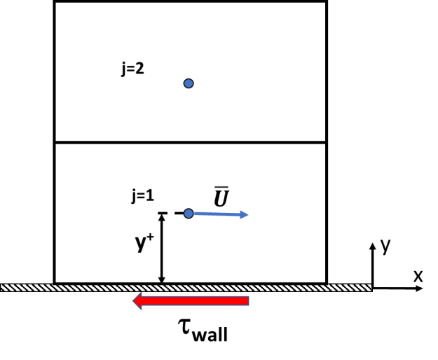
Figure 103: Near wall grid cells for a finite volume cell-centered method.
Near the wall of equilibrium flows (zero pressure gradient boundary layer, channel flow,
pipe flow, Couette flow), the solution variables follow universal laws which scale with the
wall-shear stress ?wall and the near wall molecular kinematic viscosity, ?. In other words, one
can collapse all equilibrium near wall profiles onto a single curve if the near wall variables
are non-dimensionalized by these quantities. The non-dimensionalization is based on the
wall-friction velocity  (computed from
  ), the turbulent kinetic energy
 (note that in the logarithmic layer one has
  ) and the kinematic viscosity
? in the following way:
) and the kinematic viscosity
? in the following way:
 | (12–96) |
Using these variables, one obtains a universal velocity profile of the form:
 | (12–97) |
Such profiles are depicted in Figure 104 for two Reynolds number of a boundary layer. For both Reynolds numbers, the profiles are identical near the wall and differ in the outer part. The extent to which the universal profile is followed depends on the Reynolds number.
Assuming a universal velocity profile does exist, what is the benefit for CFD? Suppose the
velocity is known in the near wall cell (j=1) e.g. from the last iteration. Since the location
of the first cell center is also known and so are the viscosity and density, they can all be
inserted into Equation (9.56). The only unknown is then the friction velocity  , which can
therefore be calculated (iteratively due to the non-linearity of the equation). From
, which can
therefore be calculated (iteratively due to the non-linearity of the equation). From  follows
the wall-shear-stress
follows
the wall-shear-stress  , which is required to close the discretization of the near
wall cell. Once this achieved, a new global iteration can be started until convergence. The
details are slightly different for each model (involving e.g.
, which is required to close the discretization of the near
wall cell. Once this achieved, a new global iteration can be started until convergence. The
details are slightly different for each model (involving e.g.  ) and can be found in the user
documentation. However, the principle is as outlined here.
) and can be found in the user
documentation. However, the principle is as outlined here.
The universal profile consists of different parts. Very close to the wall, turbulence is damped, and the velocity profile is linear (viscous sublayer). In the fully-turbulent near wall layer, the profile follows a logarithmic form (log-law). These two regions are bridged by a 'buffer layer'. This is illustrated in Figure 12.167: Universal non-dimensional velocity-profile near the wall. which depicts two flat plate boundary layer profiles (at different Reynolds numbers) in a logarithmic plot. The velocity profile can roughly be split as follows:
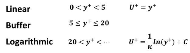
The log-profile has two constants - the von Karman constant which is typically selected to
be  and an additive constant of approximately
  .
.
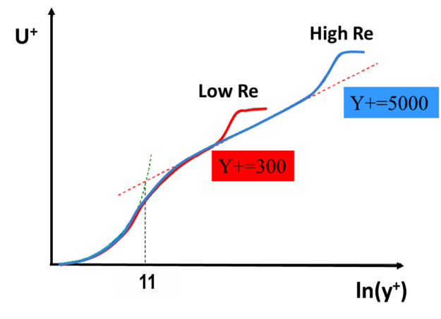
Important: while the velocity profile follows a universal law near the wall, the thickness
of the log-layer in terms of  depends on the Reynolds number. A
  resolution of say
  =50
will therefore be sufficient for a high Reynolds number flow, but not for a Low Reynolds number
flow. In the high Re case, there are plenty of cells between the wall cell and the boundary
layer edge (which is say at
=50
will therefore be sufficient for a high Reynolds number flow, but not for a Low Reynolds number
flow. In the high Re case, there are plenty of cells between the wall cell and the boundary
layer edge (which is say at  =5000), compared to a low-Re case where the boundary layer edge
might be at say
=5000), compared to a low-Re case where the boundary layer edge
might be at say  =200.
=200.
Important: Even for high Re number flows, the inner layers (sub+ buffer+ log-law) cover only 10-20% of the entire boundary layer thickness.
The following topics are discussed:
Historically, many turbulence models have been combined with a 'wall-function' (WF) approach. WF do not allow/require to integrate the equations through the viscous sublayer. Instead, the user needs to provide a grid, where the first grid point (cell center) lies in the log-layer. The wall shear stress is then computed from the log-layer formulation alone. Details of specific WF formulations can be more elaborate and can be found in the code documentation.
Wall function treatment has the advantage that simulations can be carried out on
relatively coarse grids (in wall normal direction). However, the user must ensure that the
first cell center lies in the log-layer. As depicted in Figure Figure 104, this is not trivial,
as the upper limit of the log-layer depends on the Reynolds number of the boundary layer
profile. One can therefore not define a universal upper limit, as to where the log layer is
applicable. Especially for low to moderate Reynolds number (device Re numbers of  -
- ) the
thickness of the log-layer might be narrow, and the first grid point can easily be placed
either too close or too far from the wall, missing the layer. In addition, at the lower
Reynolds numbers, even if the first cell center is placed in the log-layer, there might be not
enough resolution to cover the rest of the boundary layer with enough cells.
) the
thickness of the log-layer might be narrow, and the first grid point can easily be placed
either too close or too far from the wall, missing the layer. In addition, at the lower
Reynolds numbers, even if the first cell center is placed in the log-layer, there might be not
enough resolution to cover the rest of the boundary layer with enough cells.
Standard wall functions are highly problematic, as the solution depends on the ability of the user to:
Ensure that the cell center point is not too close to the wall so not to fall into the buffer/sublayer.
Ensure that the cell center point is not too far from the wall to not fall into the outer layer.
Ensure that the boundary layer is resolved with enough cells.
The violation of any of these conditions can result in substantial errors. Most
problematic is that mesh refinement beyond a certain level leads to a deterioration of results.
This is counter to the principles of numerical methods, where grid refinement should eventually
lead to more consistent and grid-converged solutions. The above requirements are hard to
achieve, especially at low-moderate Reynolds numbers. One needs also not to forget that the
mesh is created before a solution is available, so placing the first grid cell into the
log-layer is a difficult job. The use of standard wall functions is therefore discouraged
– it is not available when using  based models for that reason.
Users are often under the false impression that wall functions 'take care of the boundary
layer' – meaning that a grid with a properly placed  near wall cell is all that is
needed for an accurate boundary layer simulation. This is not the case. Wall functions are just
a special type of boundary conditions – the boundary layer itself still needs to be
resolved with a sufficient number of cells.
near wall cell is all that is
needed for an accurate boundary layer simulation. This is not the case. Wall functions are just
a special type of boundary conditions – the boundary layer itself still needs to be
resolved with a sufficient number of cells.
Important:
With standard wall functions, one can easily create incorrect solutions, either by overly coarse or overly fine meshes. The usage of standard wall functions is therefore not recommended.
Having a proper
 is not sufficient for accurate boundary layer simulations. One also
needs a sufficient number of cells inside the boundary layer.
is not sufficient for accurate boundary layer simulations. One also
needs a sufficient number of cells inside the boundary layer.
A simple trick can be employed to avoid the solution deterioration under mesh refinement
with standard wall functions, by applying a limiter onto  [55]:
[55]:
 | (12–98) |
This limiter prevents the wall functions to move into the viscous sublayer and thereby
guarantees a consistent wall shear-stress (and wall heat-transfer) even under mesh refinement.
While the scalable wall function is a substantial improvement, it still entails significant
assumptions, as the mesh is no longer refined towards the wall, but towards a fictitious
location at  =11, thereby slightly altering the geometry. This change is more noticeable at
low Reynolds numbers as the gap between
=11, thereby slightly altering the geometry. This change is more noticeable at
low Reynolds numbers as the gap between  =0 and
  =11 becomes a larger portion of the overall
geometry (e.g. the height of the channel or boundary layer) than for high Reynolds numbers.
=11 becomes a larger portion of the overall
geometry (e.g. the height of the channel or boundary layer) than for high Reynolds numbers.
A more consistent, albeit more expensive method is to integrate the equations all the way
to the wall. This requires a near-wall grid with a resolution of  ~1 or finer. However, such
an integration can only be performed if the turbulence models is calibrated to represent the
sublayer. Since turbulence is damped by viscosity in the buffer- and sublayer, most turbulence
models require additional damping terms and/or specific boundary conditions to account for this
effect.
~1 or finer. However, such
an integration can only be performed if the turbulence models is calibrated to represent the
sublayer. Since turbulence is damped by viscosity in the buffer- and sublayer, most turbulence
models require additional damping terms and/or specific boundary conditions to account for this
effect.
Historically models which can be integrated to the wall have been termed 'Low-Reynolds
number' models or 'low-Re' models. This is a highly confusing nomenclature, as the term
'low-Re' refers not to the device Reynolds number, but to the turbulent Reynolds number
 where
where  is the turbulent kinetic energy,
  is the wall distance and
  is the
kinematic viscosity. As
is the
kinematic viscosity. As  is damped by the presence of the wall, the turbulent kinetic energy
  approaches zero for low
  levels and so does the turbulent Re number. This is the case for all
flows close to the wall, at all device Reynolds numbers! In the following, the term 'low-Re
model' will therefore be replaced by the terminology 'Viscous Sublayer Model – VSM'.
levels and so does the turbulent Re number. This is the case for all
flows close to the wall, at all device Reynolds numbers! In the following, the term 'low-Re
model' will therefore be replaced by the terminology 'Viscous Sublayer Model – VSM'.
Developing VSMs for  -equation based models has been a major challenge. Many such models
have been developed over time (e.g. [56]), but they typically suffer from one or more of the
following deficiencies:
-equation based models has been a major challenge. Many such models
have been developed over time (e.g. [56]), but they typically suffer from one or more of the
following deficiencies:
Lack of robustness.
Multiple solutions depending on initial conditions.
Pseudo-transitional behavior not calibrated against data.
Excessive wall shear and heat transfer at reattachment/stagnation points/lines.
There are some remedies to this. The first and most widely applied is the usage of a
so-called 2-Layer formulation ([57], [58]). In this method, the epsilon equation is not solved
through the buffer and sublayer but an algebraic formulation is used instead. The  -equation is
then dominated by a source term which enforces the algebraic relations.
-equation is
then dominated by a source term which enforces the algebraic relations.
A second approach is to add additional differential equations to the  -equations based
models which account for the near wall damping. These models are typically called
'elliptic-blending' or V2F models [59]. The downside of this approach is the significantly
increased complexity due to two additional equations and the associated complex boundary
conditions. In addition, such models still allow for pseudo-transitional behavior, meaning an
artificially non-calibrated laminar-turbulent transition process, which is undesirable. For
these reasons V2F-like models are not perused in Ansys-CFD.
-equations based
models which account for the near wall damping. These models are typically called
'elliptic-blending' or V2F models [59]. The downside of this approach is the significantly
increased complexity due to two additional equations and the associated complex boundary
conditions. In addition, such models still allow for pseudo-transitional behavior, meaning an
artificially non-calibrated laminar-turbulent transition process, which is undesirable. For
these reasons V2F-like models are not perused in Ansys-CFD.
One of the strengths of the  -equation based models is that they do not require additional
damping terms. Integration to the wall can be obtained by a simple switch in boundary
conditions. These models also avoid pseudo-transition for all practical purposes and do not
lead to excessive wall shear and heat transfer at reattachment/stagnation points/lines. For
this reason,
-equation based models is that they do not require additional
damping terms. Integration to the wall can be obtained by a simple switch in boundary
conditions. These models also avoid pseudo-transition for all practical purposes and do not
lead to excessive wall shear and heat transfer at reattachment/stagnation points/lines. For
this reason,  -equation based models are the preferred option in Ansys CFD.
Important:  -equation based models are much harder to integrate to the wall than ?-based models.
Classical VSM require always a fine near wall mesh with  ~1 or smaller. This cannot be achieved for all walls in complex applications.
It is therefore desirable to be able to provide formulations which maintain consistency for a
variation in
~1 or smaller. This cannot be achieved for all walls in complex applications.
It is therefore desirable to be able to provide formulations which maintain consistency for a
variation in  . Such models are termed
  -insensitive models (or all-
 models). When computing a flow on a series of grids with different
 -resolution, such models provide wall shear-stress (and heat transfer) levels
which are approximately independent of the
-resolution, such models provide wall shear-stress (and heat transfer) levels
which are approximately independent of the  -value. Note that this statement is only correct in case of a sufficient
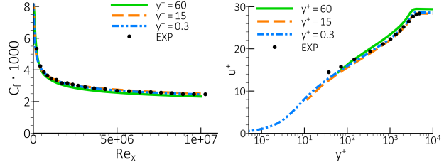
number of cells inside the boundary layer. Simulations with such a formulation can be seen in
Figure 12.168: Comparison of the skin friction coefficient and velocity profiles at
-value. Note that this statement is only correct in case of a sufficient
number of cells inside the boundary layer. Simulations with such a formulation can be seen in
Figure 12.168: Comparison of the skin friction coefficient and velocity profiles at  on different meshes for the flat plate boundary layer (28)., where a flat plate zero pressure gradient boundary layer
(28) is computed on three different grids. The computed velocity profiles follow closely the
fine grid solution. On meshes with
on different meshes for the flat plate boundary layer (28)., where a flat plate zero pressure gradient boundary layer
(28) is computed on three different grids. The computed velocity profiles follow closely the
fine grid solution. On meshes with  >20, the formulation essentially switches back to a wall function.
Figure 12.168: Comparison of the skin friction coefficient and velocity profiles at on different meshes for the flat plate boundary layer (28).
In Ansys Fluent,  -insensitive wall formulations are available for the Spalart-Allmaras
one-equation model and
-insensitive wall formulations are available for the Spalart-Allmaras
one-equation model and  models (using a 2-Layer VSM formulation and the ML VSM). In both
codes (Ansys Fluent and Ansys CFX) all
models (using a 2-Layer VSM formulation and the ML VSM). In both
codes (Ansys Fluent and Ansys CFX) all  -equations based models are based on a
  -insensitive
formulation. The details of such formulations are model and numerics dependent and are given in
more detail in the Theory Documentation of the corresponding codes.
-insensitive
formulation. The details of such formulations are model and numerics dependent and are given in
more detail in the Theory Documentation of the corresponding codes.
Y+-Insensitive Near Wall Treatment for  -based
Models
-based
Models
Near the wall, the  -equation reduces to (in the viscous sublayer production and turbulent
diffusion can also be neglected):
-equation reduces to (in the viscous sublayer production and turbulent
diffusion can also be neglected):
 | (12–99) |
This equation has the following near-wall solutions for  in the viscous sub-layer and the
log-layer:
in the viscous sub-layer and the
log-layer:
 | (12–100) |
 | (12–101) |
where  is the (typically high) value specified for
  at the wall. This formulation is
sufficient to provide proper near wall damping and the correct logarithmic layer. The
at the wall. This formulation is
sufficient to provide proper near wall damping and the correct logarithmic layer. The
 -equations
  -insensitive formulation blends smoothly between these two solutions.
The simple and robust near wall formulation without the need for complex damping functions
(or new additional transport equations like in the V2F model) makes the  model the most
attractive option as a basis for industrial turbulence models.
model the most
attractive option as a basis for industrial turbulence models.
The  Two-Layer Formulation
To avoid the complication and robustness limitations of historic VSM (low-Re)  models,
but still enable CFD users to integrate these models through the viscous sublayer, the
so-called 'two-layer' (2L) formulation was introduced [57], [58]. The 2L formulation is today
one of the more widely used turbulence near-wall formulations in industrial codes for the
models,
but still enable CFD users to integrate these models through the viscous sublayer, the
so-called 'two-layer' (2L) formulation was introduced [57], [58]. The 2L formulation is today
one of the more widely used turbulence near-wall formulations in industrial codes for the  model. Its principal idea is to avoid the complexities of the
  -equation near the wall entirely
and to replace it with an algebraic formulation, using a mixing-length model there. This
algebraic formulation is then blended with the
-equation near the wall entirely
and to replace it with an algebraic formulation, using a mixing-length model there. This
algebraic formulation is then blended with the  -equation away from the wall.
In the 2L model the near-wall  -distribution is computed from an algebraic
equation:
-distribution is computed from an algebraic
equation:
 | (12–102) |
where  is the mixing-length based on wall-distance, y:
 | (12–103) |
In addition, the eddy-viscosity is also blended between the standard  formulation and
an algebraic mixing length model:
formulation and
an algebraic mixing length model:
 | (12–104) |
Using the blending function:
 | (12–105) |
The blending is required as the distributions resulting from the algebraic formulation and
from the transport equation will not match at a pre-specified  location. To prevent
discontinuities and convergence problems, a smooth variation is required.
location. To prevent
discontinuities and convergence problems, a smooth variation is required.
The constants are:
 | (12–106) |
The turbulent Reynolds number  is also used to blend between the algebraic model and
the transport equation for
is also used to blend between the algebraic model and
the transport equation for  . The details of these blending are typically code-dependent and
are therefore not provided here. Such blending between alg. and transport equations can lead to
robustness problems and therefore needs to be performed gradually over a significant portion of
the inner portion of the boundary layer (
. The details of these blending are typically code-dependent and
are therefore not provided here. Such blending between alg. and transport equations can lead to
robustness problems and therefore needs to be performed gradually over a significant portion of
the inner portion of the boundary layer ( <200).
The 2L-blending can cause problems in low-Re number flows, where the model can be
dominated by the algebraic formulation. There is also a considerable Reynolds-number effect for
non-equilibrium flows, where the 2L mixing length model part and the  -equation produce
different results, which are then stitched together with the blending function. The relative
portion across the boundary layer where the mixing length model is active depends on the Re
number of the boundary layer. For low Re, a substantial part of the boundary layer will be
covered by the alg. part of the model, whereas for high Re, the 2L model is active only in a
small near-wall portion (relative to the boundary layer thickness). As both models behave
differently for non-equilibrium flows, this mean that the combined model will lean towards a
mixing length model for low
-equation produce
different results, which are then stitched together with the blending function. The relative
portion across the boundary layer where the mixing length model is active depends on the Re
number of the boundary layer. For low Re, a substantial part of the boundary layer will be
covered by the alg. part of the model, whereas for high Re, the 2L model is active only in a
small near-wall portion (relative to the boundary layer thickness). As both models behave
differently for non-equilibrium flows, this mean that the combined model will lean towards a
mixing length model for low  and towards a
  model for high
  .
.
Another problematic issue results from the observation that the blending function based on
 can switch back to 'near-wall mode' even outside the boundary layer in case
of low freestream values for
can switch back to 'near-wall mode' even outside the boundary layer in case
of low freestream values for  , causing non-physical distributions of the turbulence variables outside the
boundary layer. By this mechanism, a layer of high turbulence viscosity can be created
artificially, as the eddy-viscosity is also switched to the mixing length formulation (with
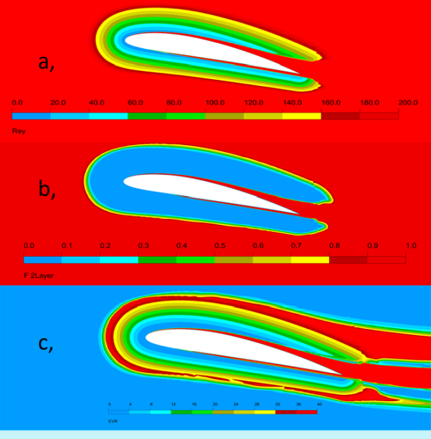
obviously a large mixing length due to the large wall distance). Figure 12.169: Contours of the
, causing non-physical distributions of the turbulence variables outside the
boundary layer. By this mechanism, a layer of high turbulence viscosity can be created
artificially, as the eddy-viscosity is also switched to the mixing length formulation (with
obviously a large mixing length due to the large wall distance). Figure 12.169: Contours of the  (Top, a,) and the Blending Function (Middle, b,) and the ratio of eddy-viscosity/molecular viscosity
  (Bottom, c,) of the 2L formulation for flow around the NACA-4412 airfoil at AoA = 12
 shows a simulation around a NACA 4412 airfoil. The
  distribution used inside the blending function is shown in part a, of the
Figure.
distribution used inside the blending function is shown in part a, of the
Figure.  is zero at the wall, increases rapidly inside the boundary layer (hard to see
in this scale), but then decreases again outside the boundary layer. The effect on the blending
function is shown in the middle Figure 106. The function is
is zero at the wall, increases rapidly inside the boundary layer (hard to see
in this scale), but then decreases again outside the boundary layer. The effect on the blending
function is shown in the middle Figure 106. The function is  =0 close to the wall (not seen on this scale) and then switches to
 =1 inside the boundary layer as desired. However, outside the boundary layer,
the formulation switches back to the algebraic form (
=1 inside the boundary layer as desired. However, outside the boundary layer,
the formulation switches back to the algebraic form ( =0). This switch-back is problematic, as it also switches the eddy-viscosity
back to the alg. formulation, which can be seen in the lower part of Figure 106c, where
=0). This switch-back is problematic, as it also switches the eddy-viscosity
back to the alg. formulation, which can be seen in the lower part of Figure 106c, where
 is plotted. This ratio reaches relatively high values outside the boundary
layer and the switches back to the low freestream values further away, as the function switches
back to
is plotted. This ratio reaches relatively high values outside the boundary
layer and the switches back to the low freestream values further away, as the function switches
back to  =1.
=1.
These examples demonstrate that the 2L model can cause issues due to its switching procedure. This is even more the case for flows with additional complexities like multi-phase flows and/or flows with large changes in physical properties, where the model has shown instabilities due to erratic switching between the mixing length and the transport equation, thereby preventing solver convergence. While the 2L formulation works well for many industrial flows, it is not strong enough to serve as a default turbulence model which needs to work for all combinations of physics.
Figure 12.169: Contours of the (Top, a,) and the Blending Function (Middle, b,) and the ratio of eddy-viscosity/molecular viscosity (Bottom, c,) of the 2L formulation for flow around the NACA-4412 airfoil at AoA = 12
In order to create a high-quality mesh, it is helpful to have some approximate formulas for
the development of boundary layers for zero pressure gradient boundary layers. The Boundary
Layer develops in streamwise direction ( -direction) for a flat plate with origin at x=0. The
boundary layer thickness is
-direction) for a flat plate with origin at x=0. The
boundary layer thickness is  , the freestream velocity is
  and the wall shear stress is
  .
The wall friction coefficient is
.
The wall friction coefficient is  and
and 
The following topics are discussed:


Wall shear stress coefficient:
 | (12–109) |
Boundary Layer thickness:
 | (12–110) |
Viscous sublayer thickness –  -estimate:
 | (12–111) |
 | (12–112) |
 | (12–113) |
This formula provides the required wall spacing  to achieve a desired
  . For
. For  it is
prudent to use half the running length of the boundary layer (e.g. half chord of an airfoil).
The good news from this equation is that
it is
prudent to use half the running length of the boundary layer (e.g. half chord of an airfoil).
The good news from this equation is that  has only a very weak variation with
  . It is
therefore possible to use a constant near wall grid spacing
. It is
therefore possible to use a constant near wall grid spacing  for the entire body. Note that
the above
for the entire body. Note that
the above  estimate is based on the grid distance between the surface and the first grid
node off the wall. The code can internally use another
estimate is based on the grid distance between the surface and the first grid
node off the wall. The code can internally use another  definition – e.g. in a
cell-centered code like Ansys Fluent it would use half of that value.
definition – e.g. in a
cell-centered code like Ansys Fluent it would use half of that value.