


The key consideration for selecting a turbulence model is the accuracy that the model can provide for a given flow, or a class of flows. As all turbulence models are more-or-less calibrated for the same base-flows (e.g. flat plate boundary layer, basic free shear flows and decaying turbulence), the model accuracy outside this narrow 'calibration box' can only be determined by further validation studies. Such studies are based on 'building block' test cases, which typically add one more element of complexity to the calibration cases, like adverse pressure gradients, separation, swirl, etc. As such cases do not account for the complex interactions seen in industrial flows, they can still not provide the full picture, but they can give a much better idea on the suitability of a model for a certain type of flows. Such tests are also the limit to which models are tested during model development and calibration, as more complex industrial flows typically lack detailed experimental data to draw meaningful conclusions on specific model deficiencies. In the following sections, model performance will be discussed for such building-block test cases, with each section focusing on a different physical effect. It is important for CFD users to understand the differences in model performance to make an educated decision during model selection.
Since this is a Best Practice Document, only the most necessary information on the test cases and their numerical set-up is provided. All solutions have been ensured to be mesh independent and, in all cases, the boundary conditions match the experiment as closely as possible.
The following topics are discussed:
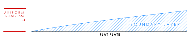
The setup of the zero pressure gradient flat plate boundary layer flow (see Figure 12.63: Schematic of the flow over a flat plate.) is based on the experiment of Wieghardt & Tillmann, [29]. The Reynolds number based on inlet velocity and the length of the
flat plate is  =
=  , and the wall is maintained at a constant temperature. No heat transfer
measurements have been carried out. Therefore, in order to assess the capability of turbulence
models to predict heat transfer to the wall, an empirical correlation is used to compute the
Stanton number at the wall from the measured distribution of skin friction coefficient.
, and the wall is maintained at a constant temperature. No heat transfer
measurements have been carried out. Therefore, in order to assess the capability of turbulence
models to predict heat transfer to the wall, an empirical correlation is used to compute the
Stanton number at the wall from the measured distribution of skin friction coefficient.
The computational domain with boundary conditions is shown in Figure 12.64: Computational domain with boundary conditions and mesh for the flow over a flat plate. Constant velocity and temperature values are assigned at the inlet plane. The difference between inlet and wall temperatures is 10° [K]. Turbulence characteristics at the inlet are also assumed constant with values corresponding to a free-stream turbulence intensity of Tu=1%, and an eddy-viscosity ratio equal to TVR=0.2. Computational meshes (see Table 1) cover three near-wall scenarios: viscous sublayer, logarithmic region and a "buffer layer" resolution.
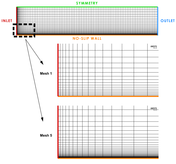
Table 12.10: Parameters of the computational meshes
|
|
Mesh 1 |
Mesh 2 |
Mesh 3 |
Mesh 4 |
Mesh 5 |
|---|---|---|---|---|---|
|
y+max |
56.9 |
22.6 |
14.4 |
3.1 |
0.3 |
|
y+mean |
33.6 |
10.9 |
6.1 |
1.1 |
0.1 |
|
Number of cells |
3800 |
4600 |
5000 |
6000 |
8000 |
Model Comparison
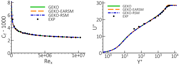
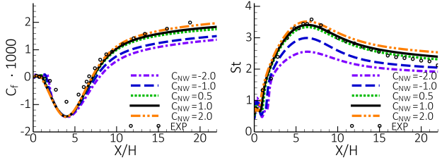
Figure 12.65: Comparison of wall shear stress coefficient, Cf (Left) and wall
heat transfer coefficient, St. (Right) for flat plate boundary layer (28) and  ~1. shows the comparison of the results of different turbulence
models (SST, GEKO, SA and RKE) on the fine mesh: Mesh-5. As expected, all the considered models
perform well for the flat plate simulations, both in terms of wall shear stress, Cf, and wall
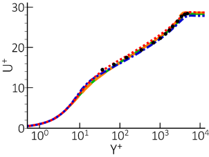
heat transfer coefficient, St, as shown in Figure 5. Also, the velocity profiles are in good
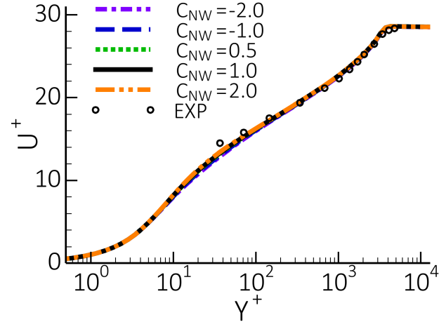
agreement with the logarithmic profile, as can be seen in Figure 12.66: Comparison of velocity profiles in wall-law for flat plate boundary layer
at Rex=8.7⋅106..
~1. shows the comparison of the results of different turbulence
models (SST, GEKO, SA and RKE) on the fine mesh: Mesh-5. As expected, all the considered models
perform well for the flat plate simulations, both in terms of wall shear stress, Cf, and wall
heat transfer coefficient, St, as shown in Figure 5. Also, the velocity profiles are in good
agreement with the logarithmic profile, as can be seen in Figure 12.66: Comparison of velocity profiles in wall-law for flat plate boundary layer
at Rex=8.7⋅106..
Figure 12.65: Comparison of wall shear stress coefficient, Cf (Left) and wall
heat transfer coefficient, St. (Right) for flat plate boundary layer (28) and ~1.
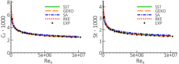
Figure 12.66: Comparison of velocity profiles in wall-law for flat plate boundary layer at Rex=8.7⋅106.
Non-linear effects
For the simple wall-bounded flows the non-linear effects of the EARSM or even RSM models do not affect the main flow. Figure 12.67: Comparison of wall shear stress coefficient (Left) and velocity profile at Rex=8.7⋅106 (Right) predicted with the GEKO model without and with EARSM/RSM options for the flat plate boundary layer (28). shows the prediction of the skin friction coefficient and wall-law velocity profile for the GEKO model without and with EARSM/RSM options.
Figure 12.67: Comparison of wall shear stress coefficient (Left) and velocity profile at Rex=8.7⋅106 (Right) predicted with the GEKO model without and with EARSM/RSM options for the flat plate boundary layer (28).
Mesh Sensitivity
For the coarser meshes, the computational accuracy depends on the wall treatment. The use
of the automatic  -insensitive wall treatment for the
  turbulence models provides virtual independence of the solution to the near
wall resolution. An example of the SST model solution is shown in Figure 12.68: Comparison of wall shear stress coefficient, Cf (upper left), wall
heat transfer coefficient, St. (upper right) and log-law velocity profile
at Rex=8.7⋅106 (lower right) for the
flat plate boundary layer using the SST model [28].. On the other hand, the accuracy of prediction of wall shear stress for high-Re
turbulence models provides virtual independence of the solution to the near
wall resolution. An example of the SST model solution is shown in Figure 12.68: Comparison of wall shear stress coefficient, Cf (upper left), wall
heat transfer coefficient, St. (upper right) and log-law velocity profile
at Rex=8.7⋅106 (lower right) for the
flat plate boundary layer using the SST model [28].. On the other hand, the accuracy of prediction of wall shear stress for high-Re
 turbulence models depends on the choice of the wall treatment. The standard
wall function (SWF) designed for the high-Re
turbulence models depends on the choice of the wall treatment. The standard
wall function (SWF) designed for the high-Re  computational grids is not adequate for the low-Re fine
  grids, as shown in Figure 12.69: Distribution of the skin friction coefficient over the flat plate computed with RKE model
with SWF (left) and ScWF (right) for the flat plate boundary layer [28]. (Left). The use of the
scalable wall function (ScWF) improves the situation considerably, as
shown in Figure 12.69: Distribution of the skin friction coefficient over the flat plate computed with RKE model
with SWF (left) and ScWF (right) for the flat plate boundary layer [28]. (Right). For the rest of the test cases, the ScWF wall
function is used for the
grids, as shown in Figure 12.69: Distribution of the skin friction coefficient over the flat plate computed with RKE model
with SWF (left) and ScWF (right) for the flat plate boundary layer [28]. (Left). The use of the
scalable wall function (ScWF) improves the situation considerably, as
shown in Figure 12.69: Distribution of the skin friction coefficient over the flat plate computed with RKE model
with SWF (left) and ScWF (right) for the flat plate boundary layer [28]. (Right). For the rest of the test cases, the ScWF wall
function is used for the  models. For the mathematical formulation of the different wall treatments see
Near-Wall Treatment.
models. For the mathematical formulation of the different wall treatments see
Near-Wall Treatment.
Figure 12.68: Comparison of wall shear stress coefficient, Cf (upper left), wall heat transfer coefficient, St. (upper right) and log-law velocity profile at Rex=8.7⋅106 (lower right) for the flat plate boundary layer using the SST model [28].
![Comparison of wall shear stress coefficient, Cf (upper left), wall heat transfer coefficient, St. (upper right) and log-law velocity profile at Rex=8.7⋅106 (lower right) for the flat plate boundary layer using the SST model [].](graphics/image020m.png)
Figure 12.69: Distribution of the skin friction coefficient over the flat plate computed with RKE model with SWF (left) and ScWF (right) for the flat plate boundary layer [28].
![Distribution of the skin friction coefficient over the flat plate computed with RKE model with SWF (left) and ScWF (right) for the flat plate boundary layer [].](graphics/image022m.png)
Figure 12.70: Distribution of the Stanton number over the flat plate computed with RKE model with SWF (left) and ScWF (right) for the flat plate boundary layer [28].
![Distribution of the Stanton number over the flat plate computed with RKE model with SWF (left) and ScWF (right) for the flat plate boundary layer [].](graphics/image024m.png)
Arguably the most important additional physical effect when developing turbulence models beyond equilibrium boundary layer flows, concerns their ability to accurately predict flows with pressure gradients and separation from smooth surfaces. This is of major importance in any external aerodynamic flow, especially airfoil and wing flows, where flow separation and stall are the defining factors of the performance envelope. However, separation from smooth surfaces is also relevant for internal flows, like diffusers and blades/vanes etc. For this reason, and because many turbulence models originate from the aeronautical community, separation prediction has always been a major focus in turbulence modeling. In more 'industrial' type flows, separation is often not caused by a pressure gradient, but by a shape change in the geometry, like a step or a corner. In such cases, the separation point/line is fixed and there is much reduced turbulence model sensitivity. This needs to be considered during the discussion of model differences for smooth wall separation. In the following 'separation' refers to separation from a smooth wall.
It is accepted knowledge in the turbulence modeling community that models are more suitable for predicting separation than models [7]. This will be demonstrated for several flows in the following
discussions. Since the Spalart-Allmaras 1-equation model is also a popular turbulence model in
aeronautics, it is included in some of the comparisons.
The following topics are discussed:
One of the most widely used test cases for evaluation of flow separation is the NASA CS0
diffuser of Driver [30], where a relatively shallow separation
region has been created in the experiment. The test case geometry (partly shown in Figure 12.71: Schematic of the flow in CS0 diffuser. near the separation zone) consists of an axisymmetric diffuser with
an internally mounted cylinder along the centerline. The boundary layer develops along the axis
of the cylinder. The expansion of the diffuser wall causes an adverse pressure gradient. The
Reynolds number based on the freestream velocity,  and the cylinder diameter
  , is equal to
  .
.
The computational domain with boundary conditions is shown in Figure 12.72: Figure 12: Computational domain with boundary conditions and mesh for CS0 diffuser.. At the inlet section, uniform streamwise velocity and turbulent quantities were specified. The outer radial boundary of the domain represents a streamline of the inviscid flow defined in the experiment, and so a free slip condition is imposed at this boundary. A no-slip condition is used on the internal cylinder wall everywhere except for the initial part where a symmetry condition is imposed (the length of the non-slip wall is adjusted to provide the correct boundary layer thickness at the first experimental section). Finally, a constant pressure condition is used at the outlet boundary.

Model Comparison
Figure 12.73: Comparison of velocity profiles predicted with different turbulence models for CS0
diffuser [30] Figure 13 shows a comparison of velocity profiles for
different turbulence models at different locations in the diffuser compared to experimental
data. The curves clearly indicate that the model family shows a strong tendency to under-predict the effect of the
adverse pressure gradient and the onset/amount of separation  . The SA is capable to reproduce negative wall shear stress, however the model
underpredicts the height of the separation bubble.
. The SA is capable to reproduce negative wall shear stress, however the model
underpredicts the height of the separation bubble.
Note that the tuned GEKO model  is an exact transformation of the standard models and therefore reproduces the model behavior which is shown in Figure 14. It is also interesting to note
that even when activating RSM (Reynolds Stress Model) model in combination with the
is an exact transformation of the standard models and therefore reproduces the model behavior which is shown in Figure 14. It is also interesting to note
that even when activating RSM (Reynolds Stress Model) model in combination with the
 -equation, the separation is still not predicted properly. Figure Figure 15
shows the wall shear-stress and the wall-pressure coefficients
-equation, the separation is still not predicted properly. Figure Figure 15
shows the wall shear-stress and the wall-pressure coefficients  and
and  for the same models. The results confirm the conclusions reached from the
velocity profiles.
for the same models. The results confirm the conclusions reached from the
velocity profiles.
It is interesting to note that family models predict firmly attached velocity profiles, even though the wall
shear stress approaches zero at around  . This is the result of the two-layer formulation (detailed described in
section 9.3.4) which allows for a very thin backflow region near the wall, even though the
overall profile is attached. This is also consistent with the distribution, which shows a lack of flow displacement for the models. Figure 16 shows the difference of the flow structure for the
based and based models.
. This is the result of the two-layer formulation (detailed described in
section 9.3.4) which allows for a very thin backflow region near the wall, even though the
overall profile is attached. This is also consistent with the distribution, which shows a lack of flow displacement for the models. Figure 16 shows the difference of the flow structure for the
based and based models.
Figure 12.73: Comparison of velocity profiles predicted with different turbulence models for CS0 diffuser [30]
![Comparison of velocity profiles predicted with different turbulence models for CS0 diffuser []](graphics/image028m.png)
Figure 12.74: Comparison of velocity profiles for k-ω model family and GEKO models for CS0 diffuser [30].
![Comparison of velocity profiles for k-ω model family and GEKO models for CS0 diffuser [].](graphics/image029m.png)
Figure 12.75: Prediction of wall characteristics for k-ω family and GEKO models for CS0 diffuser [30]. Left: wall shear stress coefficient, Cf. Right: Wall pressure coefficient Cp.
![Prediction of wall characteristics for k-ω family and GEKO models for CS0 diffuser []. Left: wall shear stress coefficient, Cf. Right: Wall pressure coefficient Cp.](graphics/image030m.png)
Figure 12.76: Flow structured visualized with the streamwise velocity field and streamlines (black lines) for CS0 diffuser [30].
![Flow structured visualized with the streamwise velocity field and streamlines (black lines) for CS0 diffuser [].](graphics/image034m.png)
GEKO Model Versatility
Variations in the CSEP coefficient for the GEKO turbulence model are shown in Figure 12.77: Figure 17: Impact of variation in ![Figure 17: Impact of variation in coefficient of the GEKO model for CS0 diffuser flow []. Left: wall shear stress coefficient, Cf. Right: Wall pressure coefficient Cp.](graphics/eqcf898f37-1022-4072-ac1e-1a8aca68794d.svg) coefficient of the GEKO model for CS0 diffuser flow [30]. Left: wall shear stress coefficient, Cf.
Right: Wall pressure coefficient Cp. - Figure 12.80: Figure 20: Impact of variation in
coefficient of the GEKO model for CS0 diffuser flow [30]. Left: wall shear stress coefficient, Cf.
Right: Wall pressure coefficient Cp. - Figure 12.80: Figure 20: Impact of variation in ![Figure 20: Impact of variation in coefficient of the GEKO model on turbulence shear stress profiles for CS0 diffuser flow [].](graphics/eqb2f283e3-a183-4060-887c-9db9f258c1ff.svg) coefficient of the GEKO model on turbulence shear
stress profiles for CS0 diffuser flow [30].. As expected, with increasing of
coefficient of the GEKO model on turbulence shear
stress profiles for CS0 diffuser flow [30].. As expected, with increasing of
 , the model becomes more sensitive to the adverse pressure gradient in the diffuser and
improves its separation predict up to a value of
, the model becomes more sensitive to the adverse pressure gradient in the diffuser and
improves its separation predict up to a value of  = 2.0. Higher values of
  lead to
over-separation. It is the desired behavior of the GEKO model to allow for a wide range of
calibration engulfing the experimental solution.
lead to
over-separation. It is the desired behavior of the GEKO model to allow for a wide range of
calibration engulfing the experimental solution.
Figure 12.77: Figure 17: Impact of variation in coefficient of the GEKO model for CS0 diffuser flow [30]. Left: wall shear stress coefficient, Cf.
Right: Wall pressure coefficient Cp.
![Figure 17: Impact of variation in coefficient of the GEKO model for CS0 diffuser flow []. Left: wall shear stress coefficient, Cf. Right: Wall pressure coefficient Cp.](graphics/image036m.png)
Figure 12.78: Figure 18: Impact of variation in ![Figure 18: Impact of variation in coefficient of the GEKO model on velocity profiles for CS0 diffuser flow [].](graphics/eq4be2da49-2545-4be4-a2be-cfda027b53d3.svg) coefficient of the GEKO model on velocity profiles for CS0 diffuser flow
[30].
coefficient of the GEKO model on velocity profiles for CS0 diffuser flow
[30].
![Figure 18: Impact of variation in coefficient of the GEKO model on velocity profiles for CS0 diffuser flow [].](graphics/image037m.png)
Figure 12.79: Figure 19: Impact of variation in ![Figure 19: Impact of variation in coefficient of the GEKO model on turbulence kinetic energy profiles for CS0 diffuser flow [].](graphics/eqc9fefdbf-7a31-4294-b2d2-892775255118.svg) coefficient of the GEKO model on turbulence
kinetic energy profiles for CS0 diffuser flow [30].
coefficient of the GEKO model on turbulence
kinetic energy profiles for CS0 diffuser flow [30].
![Figure 19: Impact of variation in coefficient of the GEKO model on turbulence kinetic energy profiles for CS0 diffuser flow [].](graphics/image038m.png)
Figure 12.80: Figure 20: Impact of variation in coefficient of the GEKO model on turbulence shear
stress profiles for CS0 diffuser flow [30].
![Figure 20: Impact of variation in coefficient of the GEKO model on turbulence shear stress profiles for CS0 diffuser flow [].](graphics/image039m.png)
Non-linear effects
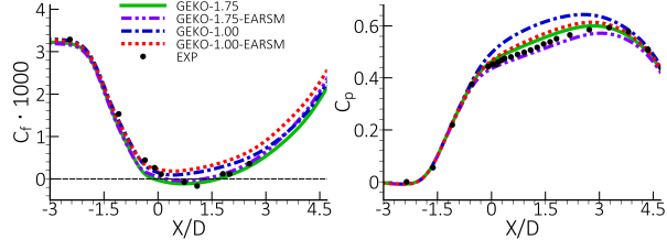
Figure 12.81: Figure 21: Impact of non-linear terms for the GEKO model for CS0 diffuser flow (30).
Left: wall shear stress coefficient, Cf. Right: Wall pressure
coefficient Cp. Figure 21 shows the results of the GEKO model with
(EARSM) and without non-linear terms. Here GEKO-1.00/1.75 corresponds to different values of
 = 1.00/1.75. Considering turbulence anisotropy of the Reynolds stress tensor has
negligible effect on the prediction of the skin friction coefficient, however the prediction of
the pressure distribution is very sensitive. The flattening of the CP-distribution indicates
that the flow is more separated when including the EARSM terms. This is expected as the EARSM
model has a similar effect as the SST limiter, by accounting for the transport of the principal
shear stress and thereby reducing the increase in the shear stress level as separation is
approached. The effect of including the EARSM formulation is therefore like an increase in
= 1.00/1.75. Considering turbulence anisotropy of the Reynolds stress tensor has
negligible effect on the prediction of the skin friction coefficient, however the prediction of
the pressure distribution is very sensitive. The flattening of the CP-distribution indicates
that the flow is more separated when including the EARSM terms. This is expected as the EARSM
model has a similar effect as the SST limiter, by accounting for the transport of the principal
shear stress and thereby reducing the increase in the shear stress level as separation is
approached. The effect of including the EARSM formulation is therefore like an increase in  for the standard GEKO model.
Figure 12.81: Figure 21: Impact of non-linear terms for the GEKO model for CS0 diffuser flow (30). Left: wall shear stress coefficient, Cf. Right: Wall pressure coefficient Cp.
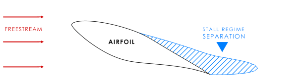
The accurate prediction of airfoil characteristics especially in regimes near stall where the flow is separated and maximal lift is achieved, is an important task for aviation and wind power, as well as for turbomachinery flows. Figure 12.82: Figure 22: Schematic of the flow around an airfoil for stall regime. shows the schematic for such a situation, where the separation zone on the suction side is significant and plays a key role in the prediction of the airfoil characteristics.
Six aerodynamic airfoils with different shapes and thicknesses (from 13% to 30%) are
considered [31]–[35].
Experimental investigations were carried out in low turbulence rectangular wind tunnels (Tu
< 1%) at relatively high Reynolds numbers (Re >  ) based on airfoil chord C and freestream velocity. The airfoil shapes and
more detailed information about the experiments are shown in the Table 12.11: Table 2: Considered airfoils and parameters of wind tunnel and flow in the
experiments. For all the airfoils, except DU-97-W-300, the boundary layer was
tripped with the use of a short rough tape placed at the leading edge. It is therefore assumed
that the flow around these airfoils is fully turbulent and that only for the "clean" DU-97-300
airfoil a model for laminar turbulent transition should be considered. For this airfoil, the
additional intermittency equation [36] is therefore solved
together with the
) based on airfoil chord C and freestream velocity. The airfoil shapes and
more detailed information about the experiments are shown in the Table 12.11: Table 2: Considered airfoils and parameters of wind tunnel and flow in the
experiments. For all the airfoils, except DU-97-W-300, the boundary layer was
tripped with the use of a short rough tape placed at the leading edge. It is therefore assumed
that the flow around these airfoils is fully turbulent and that only for the "clean" DU-97-300
airfoil a model for laminar turbulent transition should be considered. For this airfoil, the
additional intermittency equation [36] is therefore solved
together with the  and
and  -equations. Since the experimental Mach number did not exceed 0.15,
incompressible flow is assumed in all cases.
-equations. Since the experimental Mach number did not exceed 0.15,
incompressible flow is assumed in all cases.
The computations are carried out with inclusion of the wind tunnel walls. Inlet and outlet
boundaries are located 10C upstream of the leading edge and downstream of the trailing edge
airfoil, respectively. A constant velocity is specified at the inlet section of the
computational domain. No-slip conditions are used on the airfoil boundary and constant pressure
is specified at the outlet. Symmetry boundary condition are specified on the wind tunnel upper
and lower walls for imitation of slip-walls. The inlet turbulence kinetic energy matches the
experimental turbulence intensity and the specific dissipation rate is specified as  .
.
Table 12.11: Table 2: Considered airfoils and parameters of wind tunnel and flow in the experiments
|
Airfoil |
Thickness |
Surface |
Wind Tunnel Height |
Re/106 |
|---|---|---|---|---|
|
S805 |
13.5% |
Tripped |
3.60C |
1.00 |
|
S825 |
17.10% |
Tripped |
5.00C |
2.00 |
|
S809 |
21.00% |
Tripped |
3.00C |
2.00 |
|
S814 |
24.00% |
Tripped |
2.76C |
1.50 |
|
DU-97-W-180 |
18.00% |
Tripped |
3.00C |
3.00 |
|
DU-97-W-300 |
30.00% |
Clean |
3.00C |
3.00 |
|
NACA-4412 |
12.00% |
Tripped |
2.73C |
1.64 |
Model Comparison
For flows around airfoils, the maximum lift coefficient and corresponding angle of attack
are systematically overpredicted by the Reynolds Averaged Navier-Stokes (RANS) approach in
combination with standard RANS turbulence models. For example, the predicted lift coefficient
for the different turbulence models for the S809 airfoil is shown in Figure 12.83: Prediction of lift coefficient in wide range of angle of attacks for different
turbulence models for S809 airfoil at Re=![Prediction of lift coefficient in wide range of angle of attacks for different turbulence models for S809 airfoil at Re= []](graphics/eq994447a3-6439-411d-accb-85df3af5a516.svg) [33]. The disagreement between computations and experimental data is
caused by delay of turbulent boundary layer separation under adverse pressure gradient on the
suction side of the airfoils which is shown in Figure 12.83: Prediction of lift coefficient in wide range of angle of attacks for different
turbulence models for S809 airfoil at Re= [33]. Even the
most aggressive SST and GEKO (default conditions) models predict separation too late (at
[33]. The disagreement between computations and experimental data is
caused by delay of turbulent boundary layer separation under adverse pressure gradient on the
suction side of the airfoils which is shown in Figure 12.83: Prediction of lift coefficient in wide range of angle of attacks for different
turbulence models for S809 airfoil at Re= [33]. Even the
most aggressive SST and GEKO (default conditions) models predict separation too late (at
 ) while in the experiment the separation on the suction side occurs near the
mid-chord (at
) while in the experiment the separation on the suction side occurs near the
mid-chord (at  ). Since the separation position is controlled by the turbulence model, one of
the ways to improve the accuracy of the airfoil characteristics prediction is a special tuning
of the models for this class of flows.
). Since the separation position is controlled by the turbulence model, one of
the ways to improve the accuracy of the airfoil characteristics prediction is a special tuning
of the models for this class of flows.
Figure 12.83: Prediction of lift coefficient in wide range of angle of attacks for different
turbulence models for S809 airfoil at Re= [33]
![Prediction of lift coefficient in wide range of angle of attacks for different turbulence models for S809 airfoil at Re= []](graphics/image041edit.png)
GEKO Model Tuning
The simplest way of model turning without violating the basic flows calibration is to
increase the  coefficient of the GEKO model. This coefficient (default value is
 =1.75) affects the size of separation bubble: for higher
  values the separation is larger. Figure 12.84: Prediction of lift and pressure coefficients with GEKO model for DU-96-W-180 [35] (Left) and DU-97-W-300 [35] (Right)
airfoil at Re=
values the separation is larger. Figure 12.84: Prediction of lift and pressure coefficients with GEKO model for DU-96-W-180 [35] (Left) and DU-97-W-300 [35] (Right)
airfoil at Re=![Prediction of lift and pressure coefficients with GEKO model for DU-96-W-180 [] (Left) and DU-97-W-300 [] (Right) airfoil at Re=](graphics/eq59c7ce75-2256-470e-a046-f5c928bb84e3.svg)
 Figure 12.88: Prediction of lift coefficient in wide range of angle of attacks (Left) and pressure
coefficient for
Figure 12.88: Prediction of lift coefficient in wide range of angle of attacks (Left) and pressure
coefficient for ![Prediction of lift coefficient in wide range of angle of attacks (Left) and pressure coefficient for (Right) with GEKO model for S814 airfoil at Re= []](graphics/eq6b0339e2-1d3f-4097-a1dc-d61632371f89.svg) (Right) with GEKO model for S814 airfoil at Re=
(Right) with GEKO model for S814 airfoil at Re=![Prediction of lift coefficient in wide range of angle of attacks (Left) and pressure coefficient for (Right) with GEKO model for S814 airfoil at Re= []](graphics/eq43c51b8d-ac9a-4622-b0d3-1598bb6c63a6.svg) [34] compare lift curves for 1.75
[34] compare lift curves for 1.75
 2.5 for all the considered airfoils. In these comparisons, it should be kept
in mind that 2D simulations are not correct in the post-stall region, due to the formation of
3D structures in the experiments [37]. Despite this, it is
possible to adjust the GEKO model for the prediction of such flows for angles of attack up to
stall using 2D simulations. The GEKO-2.50 (GEKO with
2.5 for all the considered airfoils. In these comparisons, it should be kept
in mind that 2D simulations are not correct in the post-stall region, due to the formation of
3D structures in the experiments [37]. Despite this, it is
possible to adjust the GEKO model for the prediction of such flows for angles of attack up to
stall using 2D simulations. The GEKO-2.50 (GEKO with  = 2.5) model predicts earlier separation on the suction side of the airfoils
than other model variants, which improves agreement of the predicted both integral (lift
coefficient) and local (pressure coefficient) airfoil characteristics with the experimental
data near stall. However, the GEKO-2.50 model underpredicts the lift coefficient for low angles
of attack for the thickest DU-97-W-300 and S814 airfoils (30% thickness) which is undesirable.
The optimal
= 2.5) model predicts earlier separation on the suction side of the airfoils
than other model variants, which improves agreement of the predicted both integral (lift
coefficient) and local (pressure coefficient) airfoil characteristics with the experimental
data near stall. However, the GEKO-2.50 model underpredicts the lift coefficient for low angles
of attack for the thickest DU-97-W-300 and S814 airfoils (30% thickness) which is undesirable.
The optimal  value is therefore between
  =2.00-2.50.
Figure 12.84: Prediction of lift and pressure coefficients with GEKO model for DU-96-W-180 [35] (Left) and DU-97-W-300 [35] (Right)
airfoil at Re=
![Prediction of lift and pressure coefficients with GEKO model for DU-96-W-180 [] (Left) and DU-97-W-300 [] (Right) airfoil at Re=](graphics/image040.png)
Figure 12.85: Prediction of lift coefficient in wide range of angle of attacks (Left) and pressure
coefficient for ![Prediction of lift coefficient in wide range of angle of attacks (Left) and pressure coefficient for (Right) with GEKO model for S805 airfoil at Re=1 []](graphics/eqba889708-9bde-4a87-8f57-baa5d74c4df0.svg) (Right) with GEKO model for S805 airfoil at Re=1
(Right) with GEKO model for S805 airfoil at Re=1![Prediction of lift coefficient in wide range of angle of attacks (Left) and pressure coefficient for (Right) with GEKO model for S805 airfoil at Re=1 []](graphics/eq50a51f26-5b7b-457b-9bc8-6b774a1e4f8d.svg)
![Prediction of lift coefficient in wide range of angle of attacks (Left) and pressure coefficient for (Right) with GEKO model for S805 airfoil at Re=1 []](graphics/eq35aad57c-677c-4d9b-8969-6e7d55075d3c.svg) [31]
[31]
![Prediction of lift coefficient in wide range of angle of attacks (Left) and pressure coefficient for (Right) with GEKO model for S805 airfoil at Re=1 []](graphics/image047.png)
Figure 12.86: Prediction of lift coefficient in wide range of angle of attacks (Left) and pressure
coefficient for ![Prediction of lift coefficient in wide range of angle of attacks (Left) and pressure coefficient for (Right) with GEKO model for S825 airfoil at Re= []](graphics/eqb3d2b7fd-07f2-42fc-b5d5-75662ab19193.svg) (Right) with GEKO model for S825 airfoil at Re=
(Right) with GEKO model for S825 airfoil at Re=![Prediction of lift coefficient in wide range of angle of attacks (Left) and pressure coefficient for (Right) with GEKO model for S825 airfoil at Re= []](graphics/eq443f3c34-a12b-4d56-85e8-d9dcce4496ae.svg) [32]
[32]
![Prediction of lift coefficient in wide range of angle of attacks (Left) and pressure coefficient for (Right) with GEKO model for S825 airfoil at Re= []](graphics/image048.png)
Figure 12.87: Prediction of lift coefficient in wide range of angle of attacks (Left) and pressure
coefficient for ![Prediction of lift coefficient in wide range of angle of attacks (Left) and pressure coefficient for (Right) with GEKO model for S809 airfoil at Re= []](graphics/eqd282412f-cb1e-40dc-a355-c93b24eddc70.svg) (Right) with GEKO model for S809 airfoil at Re=
(Right) with GEKO model for S809 airfoil at Re=![Prediction of lift coefficient in wide range of angle of attacks (Left) and pressure coefficient for (Right) with GEKO model for S809 airfoil at Re= []](graphics/eq0c95e89e-4450-40cc-bc1f-9f9b0b805126.svg) [33]
[33]
![Prediction of lift coefficient in wide range of angle of attacks (Left) and pressure coefficient for (Right) with GEKO model for S809 airfoil at Re= []](graphics/image049.png)
Figure 12.88: Prediction of lift coefficient in wide range of angle of attacks (Left) and pressure
coefficient for (Right) with GEKO model for S814 airfoil at Re= [34]
![Prediction of lift coefficient in wide range of angle of attacks (Left) and pressure coefficient for (Right) with GEKO model for S814 airfoil at Re= []](graphics/image050.png)
Non-linear effects
An example of considering non-linear effects for the GEKO model using an EARSM model is
presented next. Figure 12.89: NACA-4412 airfoil near the trailing edge with streamwise velocity profiles at
measurement locations predicted with linear and non-linear GEKO-1.75 model compared with the
experimental data [38] shows the effect of the non-linear WJ-EARSM
terms for the NACA-4412 airfoil for the GEKO-1.75 (  = 1.75) model. The use of the non-linear terms slightly increases separation
on the suction side of the airfoils. However, the effect is much weaker than the model tuning
with the
= 1.75) model. The use of the non-linear terms slightly increases separation
on the suction side of the airfoils. However, the effect is much weaker than the model tuning
with the  coefficient shown above.
Figure 12.89: NACA-4412 airfoil near the trailing edge with streamwise velocity profiles at measurement locations predicted with linear and non-linear GEKO-1.75 model compared with the experimental data [38]
![NACA-4412 airfoil near the trailing edge with streamwise velocity profiles at measurement locations predicted with linear and non-linear GEKO-1.75 model compared with the experimental data []](graphics/image051.png)
Transonic compressible flow past an axisymmetric bump was simulated at conditions corresponding to the experiments of Bachalo & Johnson [39]. The bump was placed over a cylindrical pipe, and the entire geometry is axisymmetric. The incoming Reynolds number based on the bump chord length was Re = 2.763⋅106. The dynamic viscosity was assumed to adhere to Sutherland's law and the Prandtl number was set to Pr = 0.71.
The NASA Bump flow features a subsonic inflow with Ma=0.875. The flow is then accelerated to supersonic speed over the bump and then reverts to subsonic speed through a shock wave. The shock causes the boundary layer behind the shock to separate, which in turn interacts with the shock by pushing it forward. The ability to predict the shock location is therefore directly linked to a model's ability to predict boundary layer separation.
The size of the computational domain as illustrated in Figure 12.91: Computational domain with boundary conditions and mesh for the NASA Transonic Bump
[39]
was about 12C by 4C (C is the bump length). The inlet boundary is located 6.89C upstream of the
bump. Constant total pressure of  = 106595 [Pa] and total temperature of
  = 322 [K] are assigned at the inlet section of the computational domain.
Turbulence characteristics over the inlet are also assumed constant with values corresponding
to a free-stream turbulence intensity of Tu=0.1%, and an eddy-viscosity ratio of TVR=1. A
no-slip condition is used on the wall and a constant pressure is specified at the outlet
boundary. The computational mesh shown in Figure 12.91: Computational domain with boundary conditions and mesh for the NASA Transonic Bump
[39] is refined in
streamwise direction over the bump for proper resolution of the shock wave.
= 322 [K] are assigned at the inlet section of the computational domain.
Turbulence characteristics over the inlet are also assumed constant with values corresponding
to a free-stream turbulence intensity of Tu=0.1%, and an eddy-viscosity ratio of TVR=1. A
no-slip condition is used on the wall and a constant pressure is specified at the outlet
boundary. The computational mesh shown in Figure 12.91: Computational domain with boundary conditions and mesh for the NASA Transonic Bump
[39] is refined in
streamwise direction over the bump for proper resolution of the shock wave.
Figure 12.91: Computational domain with boundary conditions and mesh for the NASA Transonic Bump [39]
![Computational domain with boundary conditions and mesh for the NASA Transonic Bump []](graphics/image053.png)
As expected, again, the models form two groups with GEKO-1.75/SST and GEKO-1.00/RKE as
seen from Figure 12.92: Comparison of wall pressure coefficient, ![Comparison of wall pressure coefficient, for the transonic bump flow []. The bump starts at =0 location. Left: comparison of the different turbulence models, right: versatility of the GEKO model with the variation (GEKO-1.75: =1.75)](graphics/eq5725d3f4-8ba3-4a4a-b6ff-77d6a5127568.svg) for the transonic bump flow [39]. The bump
starts at
for the transonic bump flow [39]. The bump
starts at ![Comparison of wall pressure coefficient, for the transonic bump flow []. The bump starts at =0 location. Left: comparison of the different turbulence models, right: versatility of the GEKO model with the variation (GEKO-1.75: =1.75)](graphics/eq7bdcda2f-88db-4a54-a79b-cd04fd2c759a.svg) =0 location. Left: comparison of the different turbulence models, right:
versatility of the GEKO model with the
=0 location. Left: comparison of the different turbulence models, right:
versatility of the GEKO model with the ![Comparison of wall pressure coefficient, for the transonic bump flow []. The bump starts at =0 location. Left: comparison of the different turbulence models, right: versatility of the GEKO model with the variation (GEKO-1.75: =1.75)](graphics/eq159ed8f8-9cd2-4652-9cf2-0383f2a3ceb0.svg) variation (GEKO-1.75:
variation (GEKO-1.75: ![Comparison of wall pressure coefficient, for the transonic bump flow []. The bump starts at =0 location. Left: comparison of the different turbulence models, right: versatility of the GEKO model with the variation (GEKO-1.75: =1.75)](graphics/eq79313739-c09c-4d82-89fd-a8a19f652e72.svg) =1.75). Only the GEKO-1.75/SST model can predict the shock location and the
post-shock separation zone properly. The GEKO-1.00/RKE models fail due to their lack of
separation sensitivity. Like for the other described cases, the non-linear terms show less
influence on the size of separation zone than the choice of the turbulence model, Figure 12.93: Comparison of different
=1.75). Only the GEKO-1.75/SST model can predict the shock location and the
post-shock separation zone properly. The GEKO-1.00/RKE models fail due to their lack of
separation sensitivity. Like for the other described cases, the non-linear terms show less
influence on the size of separation zone than the choice of the turbulence model, Figure 12.93: Comparison of different ![Comparison of different settings and ERSM inclusion for the transonic bump flow []. Left: wall shear stress coefficient, , right: wall pressure stress coefficient](graphics/eq17ae92f7-8d28-4964-a652-8586119b9792.svg) settings and ERSM inclusion for the transonic bump flow [39]. Left: wall shear stress coefficient,
settings and ERSM inclusion for the transonic bump flow [39]. Left: wall shear stress coefficient, ![Comparison of different settings and ERSM inclusion for the transonic bump flow []. Left: wall shear stress coefficient, , right: wall pressure stress coefficient](graphics/eq15658f51-7d93-4495-9145-9be51eed9c6f.svg) , right: wall pressure stress coefficient
, right: wall pressure stress coefficient ![Comparison of different settings and ERSM inclusion for the transonic bump flow []. Left: wall shear stress coefficient, , right: wall pressure stress coefficient](graphics/eq17404648-a7d9-4dda-b014-05940f01fa56.svg) .
.
Figure 12.92: Comparison of wall pressure coefficient, for the transonic bump flow [39]. The bump
starts at =0 location. Left: comparison of the different turbulence models, right:
versatility of the GEKO model with the variation (GEKO-1.75: =1.75)
![Comparison of wall pressure coefficient, for the transonic bump flow []. The bump starts at =0 location. Left: comparison of the different turbulence models, right: versatility of the GEKO model with the variation (GEKO-1.75: =1.75)](graphics/image054.5.png)
Figure 12.93: Comparison of different settings and ERSM inclusion for the transonic bump flow [39]. Left: wall shear stress coefficient, , right: wall pressure stress coefficient
![Comparison of different settings and ERSM inclusion for the transonic bump flow []. Left: wall shear stress coefficient, , right: wall pressure stress coefficient](graphics/image056.5.png)
As described in section 3.4.3, eddy-viscosity models need special corrections for the
prediction of the secondary flows in corners. In this section, the effect of the use of CFC
(Corner flow Correction) [22], [23]
and EARSM terms from the Wallin-Johansson [19] model (see section
3.3.3) in combination with different  models is shown for flows in rectangular channels and diffusers. For these
flows, only the inclusion of the non-linear terms allows to predict the secondary flows in the
corners.
models is shown for flows in rectangular channels and diffusers. For these
flows, only the inclusion of the non-linear terms allows to predict the secondary flows in the
corners.
Thus, the main goal of this section is to demonstrate the improvement in the prediction of the secondary motion in corners with the use of the non-linear turbulence models. The non-linear effects are shown for the GEKO model in combination the Corner Flow Correction (CFC) and EARSM. The effect of these terms on other models like the SST model would be similar.
The following topics are discussed:
The simplest case demonstrating the impact of the secondary motion on the main flow is the developed flow in square duct. For this flow, the linear eddy-viscosity models are not capable to predict secondary motion into the corners. This effect is shown in Figure 12.94: Flow topology in the square duct case predicted using the GEKO model with CFC (left) and without CFC (right). Blue lines: iso-surfaces of the streamwise velocity, red lines in the corners: streamlines of the secondary motion.
Figure 12.94: Flow topology in the square duct case predicted using the GEKO model with CFC (left) and without CFC (right). Blue lines: iso-surfaces of the streamwise velocity, red lines in the corners: streamlines of the secondary motion
The computations are performed with the linear and non-linear GEKO-CFC model under the
conditions of the reference DNS data [40], namely at a Reynolds
number based on the averaged friction velocity  and the channel width,
  , equal to
  =1200. The computations were carried out in a "2.5D mode", which include
momentum equations for all the 3 velocity components but assumed that their streamwise
derivatives are zero. A constant streamwise pressure gradient is specified to achieve the DNS
Reynolds number. At solid walls, no-slip boundary conditions are imposed.
=1200. The computations were carried out in a "2.5D mode", which include
momentum equations for all the 3 velocity components but assumed that their streamwise
derivatives are zero. A constant streamwise pressure gradient is specified to achieve the DNS
Reynolds number. At solid walls, no-slip boundary conditions are imposed.
The streamlines in the cross-section show that the non-linear GEKO model can predict secondary flow while the linear GEKO model cannot (see Figure 12.94: Flow topology in the square duct case predicted using the GEKO model with CFC (left) and without CFC (right). Blue lines: iso-surfaces of the streamwise velocity, red lines in the corners: streamlines of the secondary motion). The flow structure of GEKO-1.00, GEKO-1.75 and WJ-BSL-EARSM model is virtually the same (not shown). Streamwise and lateral velocity profiles along a diagonal line (X=Y) predicted by the GEKO-EARSM models are in reasonable agreement with the DNS data (see Figure 12.95: Streamwise (Left) and lateral (Right) velocity profiles on the diagonal of the square duct case [40]).
Figure 12.95: Streamwise (Left) and lateral (Right) velocity profiles on the diagonal of the square duct case [40]
![Streamwise (Left) and lateral (Right) velocity profiles on the diagonal of the square duct case []](graphics/image060.5.png)
Flow in rectangular diffusers is a much more challenging test case than the fully developed channel flow, since it involves the effect of turbulence anisotropy combined with an adverse pressure gradient causing separation of the flow. Two diffusers are considered: the symmetric DLR diffuser [41] and the asymmetric Stanford diffuser [42], [43] where the flow is highly sensitive to the secondary flow prediction.
DLR-Diffuser
Flow is modeled based on the experimental study in the framework of DLR project  to investigate 3D separated flow, which occur at end wall junctions. The diffuser configuration
with the expansion ratio of ER = 2.0 was considered in the CFD study is shown in Figure Figure
36. Computational domain together with boundary conditions is shown in Figure 12.97: Computational domain with the boundary conditions for the DLR diffuser [41]. The
inlet condition is unform flow with U=10m/s Tu=1% and TVR=1. A no-slip condition is used at the
wall and a constant pressure is specified at the outlet boundary. The origin the of coordinate
system is located on the centerline of the flat wall coincident with the start of the ramp. The
X-axis is aligned with the streamwise direction, the Y-axis defines the spanwise direction
while the Z-axis coincides with the expansion direction of the channel. Reynolds number based
on the inlet bulk velocity and cross-section of internal width
to investigate 3D separated flow, which occur at end wall junctions. The diffuser configuration
with the expansion ratio of ER = 2.0 was considered in the CFD study is shown in Figure Figure
36. Computational domain together with boundary conditions is shown in Figure 12.97: Computational domain with the boundary conditions for the DLR diffuser [41]. The
inlet condition is unform flow with U=10m/s Tu=1% and TVR=1. A no-slip condition is used at the
wall and a constant pressure is specified at the outlet boundary. The origin the of coordinate
system is located on the centerline of the flat wall coincident with the start of the ramp. The
X-axis is aligned with the streamwise direction, the Y-axis defines the spanwise direction
while the Z-axis coincides with the expansion direction of the channel. Reynolds number based
on the inlet bulk velocity and cross-section of internal width  is Re =
For this case, the linear models predict two recirculation zones starting from the
inclined-side wall corner as shown in Figure 12.98: The surface streamlines near the inclined and side walls plotted for the linear (left)
and non-linear GEKO model with corner flow correction (right) for the DLR diffuser [41]. Figure 12.99: Flow topology for the linear (left) and non-linear GEKO model with corner flow
correction (right) for the DLR diffuser [41]. In contrast, the secondary flow predicted
with non-linear model prevents corner separation and pushes the recirculation zone to the
inclined wall, while flow on the side wall is virtually attached. The dramatic difference in
flow topology, visualized by the wall-streamlines on the inclined wall with the linear and
non-linear GEKO model is shown in Figure 12.98: The surface streamlines near the inclined and side walls plotted for the linear (left)
and non-linear GEKO model with corner flow correction (right) for the DLR diffuser [41].
Figure 12.99: Flow topology for the linear (left) and non-linear GEKO model with corner flow
correction (right) for the DLR diffuser [41]. In contrast, the secondary flow predicted
with non-linear model prevents corner separation and pushes the recirculation zone to the
inclined wall, while flow on the side wall is virtually attached. The dramatic difference in
flow topology, visualized by the wall-streamlines on the inclined wall with the linear and
non-linear GEKO model is shown in Figure 12.98: The surface streamlines near the inclined and side walls plotted for the linear (left)
and non-linear GEKO model with corner flow correction (right) for the DLR diffuser [41]. Figure 12.99: Flow topology for the linear (left) and non-linear GEKO model with corner flow
correction (right) for the DLR diffuser [41] .
Figure 12.99: Flow topology for the linear (left) and non-linear GEKO model with corner flow
correction (right) for the DLR diffuser [41] .
![DLR diffuser configuration []](graphics/image062.png)
![Computational domain with the boundary conditions for the DLR diffuser []](graphics/image063.png)
A comparison of the predicted skin friction coefficient with the experimental data (Figure 12.100: Distribution of the skin friction along the diffuser at midsection (left) and near the corner (right) for turbulence models with and without non-linear terms for the DLR diffuser [41]) shows that the use of the non-linear models improves the prediction of the flow near the corner (y/h=0.46) where the linear models predict large corner separations. In contrast, the flow near the midsection (y/h=0) of the diffuser in not so sensitive to the non-linear effects. However, all the models predict an attached boundary layer at the midsection, while in the experiment the flow separates. Despite the different flow topologies for linear and non-linear models, the pressure distribution at the midsection (Figure 12.101: Distribution of the pressure coefficient along the diffuser at midsection for turbulence models with and without non-linear terms for the DLR diffuser [41]) agrees with the experimental data for all the models.
Figure 12.98: The surface streamlines near the inclined and side walls plotted for the linear (left) and non-linear GEKO model with corner flow correction (right) for the DLR diffuser [41].
![The surface streamlines near the inclined and side walls plotted for the linear (left) and non-linear GEKO model with corner flow correction (right) for the DLR diffuser [].](graphics/image064.5.png)
Figure 12.99: Flow topology for the linear (left) and non-linear GEKO model with corner flow correction (right) for the DLR diffuser [41]
![Flow topology for the linear (left) and non-linear GEKO model with corner flow correction (right) for the DLR diffuser []](graphics/image065.1.png)
Figure 12.100: Distribution of the skin friction along the diffuser at midsection (left) and near the corner (right) for turbulence models with and without non-linear terms for the DLR diffuser [41]
![Distribution of the skin friction along the diffuser at midsection (left) and near the corner (right) for turbulence models with and without non-linear terms for the DLR diffuser []](graphics/image068.5.png)
Figure 12.101: Distribution of the pressure coefficient along the diffuser at midsection for turbulence models with and without non-linear terms for the DLR diffuser [41]
![Distribution of the pressure coefficient along the diffuser at midsection for turbulence models with and without non-linear terms for the DLR diffuser []](graphics/image070.5.png)
Stanford Diffuser
This flow studied experimentally by Cherry et al. [42], [43] is even more challenging than the flows considered above. For this case, separation has proven very sensitive to details of turbulence modeling. It seems clear that the anisotropy of the normal stresses must be accounted for to avoid the formation of an incorrect flow topology.
The geometry of the diffuser is shown in Figure 12.102: Geometry of Stanford diffuser [42], [43].. The top wall of the diffuser is inclined by an angle of 11.3 degrees. To achieve asymmetry, one the side walls is inclined by 2.56 degrees. The coordinate system used in the computations is shown in Figure 12.103: Computational domain with boundary conditions for the Stanford diffuser [42], [43].. The origin of the coordinate system in the X-direction is located at the cross-section of the diffuser corresponding to the intersection of its straight and inclined walls in the Y- and Z-directions; it is in the vertex of the dihedral angle formed by the straight walls of the diffuser.
In accordance with the experimental setup, the inlet flow is considered as fully developed
flow in a rectangular duct with the bulk velocity providing a Reynolds number of Re =  . The
velocity in the inlet plane is specified using precursor computations of the developed
rectangular channel flow with the same turbulence model used later for the diffuser simulation.
The computations were carried out with the GEKO model with and without corner flow correction
(CFC), GEKO-EARSM model and differential Reynold-Stress GEKO model (GEKO-RSM).
. The
velocity in the inlet plane is specified using precursor computations of the developed
rectangular channel flow with the same turbulence model used later for the diffuser simulation.
The computations were carried out with the GEKO model with and without corner flow correction
(CFC), GEKO-EARSM model and differential Reynold-Stress GEKO model (GEKO-RSM).
![Geometry of Stanford diffuser [], [].](graphics/image072.png)
![Computational domain with boundary conditions for the Stanford diffuser [], [].](graphics/image073.png)
Figure 12.104: Flow topology for the linear (left) and non-linear CFC-GEKO model (middle) for the Stanford diffuser. Experimental data (right) [42], [43]. shows the 3D flow topology for the linear, the
non-linear GEKO model and the experiment (note that these pictures are turned by 180° for
visualization purposes). It is well seen that in the experiment the separation occurs mainly on
the strongly inclined wall. The linear GEKO model predicts massive corner separation in the
expanding part of the diffuser and separation occurs on the non-inclined side wall. The
non-linear model decreases the size of the corner separation zone which dramatically changes
the flow topology. For the non-linear model, the separation occurs mainly on the strongly
inclined wall which is in better agreement with the experimental flow topology. The effects of
the nonlinearity on the flow topology are also shown on Figure 12.105: Streamwise velocity contours predicted by the linear and non-linear GEKO ( =1.00) model at X5 section. Blue colors indicate recirculation zone.
where the streamwise velocity contours at section X5 are plotted (blue colors indicates
negative values). The non-linear terms change the separation zone location (from the side wall
to the inclined wall). The results of all the non-linear models are close to each other.
=1.00) model at X5 section. Blue colors indicate recirculation zone.
where the streamwise velocity contours at section X5 are plotted (blue colors indicates
negative values). The non-linear terms change the separation zone location (from the side wall
to the inclined wall). The results of all the non-linear models are close to each other.
Figure 12.104: Flow topology for the linear (left) and non-linear CFC-GEKO model (middle) for the Stanford diffuser. Experimental data (right) [42], [43].
![Flow topology for the linear (left) and non-linear CFC-GEKO model (middle) for the Stanford diffuser. Experimental data (right) [], [].](graphics/image074.5.png)
Figure 12.105: Streamwise velocity contours predicted by the linear and non-linear GEKO (=1.00) model at X5 section. Blue colors indicate recirculation zone.
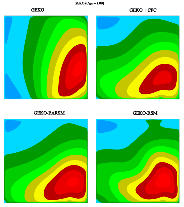
Interestingly, the flow topology for the non-linear models also depends on the baseline
linear model. Figure 12.106: Streamwise velocity contours predicted be the linear and non-linear GEKO ( =1.75) model at X5 section. Blue colors indicate recirculation zone. shows that the increase of
  in the GEKO model from
  = 1.00 to CSEP = 1.75 leads a separation on both, the side and inclined wall.
The effect of the
= 1.00 to CSEP = 1.75 leads a separation on both, the side and inclined wall.
The effect of the  value on the prediction of the pressure coefficient is shown in Figure 12.107: Distribution of the pressure coefficient along the diffuser at midsection for turbulence models with and without non-linear terms for the Stanford diffuser [42], [43].. As seen, the more aggressive
  settings (higher
  ) fail to capture the overall pressure distribution.
As the tests indicate, this flow is extremely sensitive to modeling details, as it allows
for topology changes in the solution based on model settings. Poor results are obtained for
 =1.75, as typically chosen for aerodynamic flows. This might be a result of the large
separation zone predicted by the model. Such zones tend to be poorly predicted by RANS as the
reattachment dynamics can be dominated by small-scale shedding from the separation line. As
such effects are not included in RANS, it can lead to overly large separation zones. The error
can be reduced by more conservative settings e.g. for
=1.75, as typically chosen for aerodynamic flows. This might be a result of the large
separation zone predicted by the model. Such zones tend to be poorly predicted by RANS as the
reattachment dynamics can be dominated by small-scale shedding from the separation line. As
such effects are not included in RANS, it can lead to overly large separation zones. The error
can be reduced by more conservative settings e.g. for  =1, which delays separation and
thereby reduces the separation zone. While giving a better overall agreement with data, it
could be the result of a cancelation of errors. This example shows that seemingly simple
experimental configurations can still pose severe challenges to RANS modeling.
=1, which delays separation and
thereby reduces the separation zone. While giving a better overall agreement with data, it
could be the result of a cancelation of errors. This example shows that seemingly simple
experimental configurations can still pose severe challenges to RANS modeling.
Figure 12.106: Streamwise velocity contours predicted be the linear and non-linear GEKO (=1.75) model at X5 section. Blue colors indicate recirculation zone.
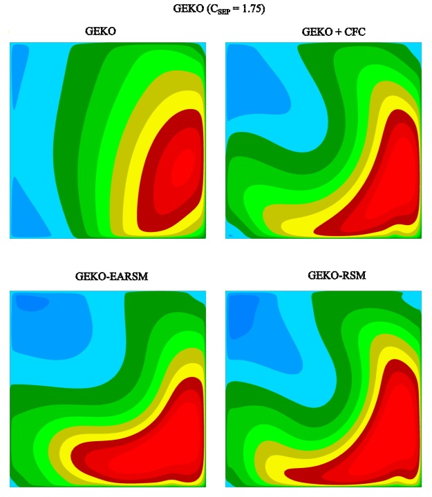
Figure 12.107: Distribution of the pressure coefficient along the diffuser at midsection for turbulence models with and without non-linear terms for the Stanford diffuser [42], [43].
![Distribution of the pressure coefficient along the diffuser at midsection for turbulence models with and without non-linear terms for the Stanford diffuser [], [].](graphics/image084.5.png)
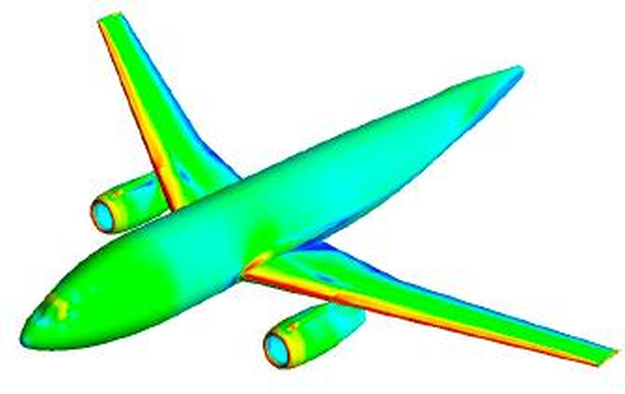
Transonic flow past the DLR F6 airplane configuration with mounted engine shown in Figure Figure 48 at Mach number of Ma = 0.75 and Re = 3⋅106 was considered. The variant for the geometry with mounted engine was selected for comparison, with an angle of attack of 1 degree, providing a lift coefficient of about CL=0.5. Computations were performed in the Ansys CFX on a block-structured grid of 8.4 million elements. References to the measurement carried out at ONERA are available in 2nd AIAA CFD drag prediction workshop (https://aiaa-dpw.larc.nasa.gov/Workshop2/workshop2.html).
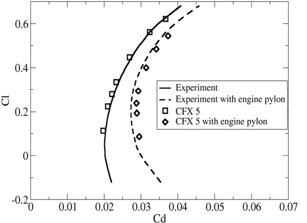
The main challenge in the workshop was to predict the drag differences between a wing-body without and with the engine-nacelle installed. Figure 12.109: Lift-Drag Polar for Wing body without and with engine pylon + nacelle shows the lift-drag polar (different points are for different angles of attack) using the SST model. As can be seen, the data were very well represented in the simulations.
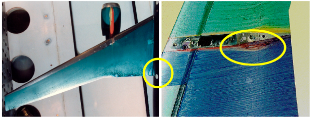
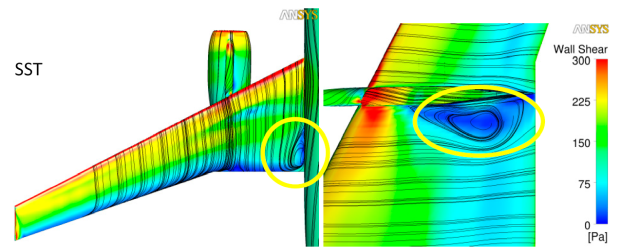
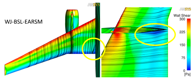
However, in the current section, the interest is more in the details of the corners flows and the effect of non-linear models in such areas. The SST model tends to overpredict the size of the corner separation zones, due to the lack of secondary flow prediction in the corner, as shown in Figure 12.110: Separation zone at the upper wing-fuselage junction (left) and lower wing surface behind the engine (right). Top - oil film visualization in the experiment.. The WJ-BSL-EARSM model improves the result for the wing-fuselage corner separation on the upper wing surface (left set of pictures in Figure 12.110: Separation zone at the upper wing-fuselage junction (left) and lower wing surface behind the engine (right). Top - oil film visualization in the experiment.). The other corner separation zone sits on the lower wing surface where the engine is mounted to the wing. The separation there is also over-predicted by the SST model. With the WJ-BSL-EARSM model, the separation size is substantially diminished in agreement with the experiment.
Figure 12.110: Separation zone at the upper wing-fuselage junction (left) and lower wing surface behind the engine (right). Top - oil film visualization in the experiment.
Non-linear effects play a significant role for the flows with secondary motions in corners. Linear eddy-viscosity models fail to predict the correct flow topology in the corners. For flows with pressure gradient and separation, this can lead to incorrect predictions of the flow topology. Non-linear models like CFC or EARSM formulations, significantly improve predictions of such flows. The use of the differential Reynolds Stress models does not lead to a significantly further improvement in comparison with the EARSM model.
This section shows two examples of the use of the curvature correction (described above in section 3.4.2): flow in a hydro-cyclone and a NACA-0012 wing tip vortex flow. For both cases, the curvature correction is used in combination with the SST model (SST-CC).
The following topics are discussed:
The NACA 0012 wing tip vortex test case is based on the experiment of Chow et al. [44].
There is a number of detailed experimental data available at various downstream locations
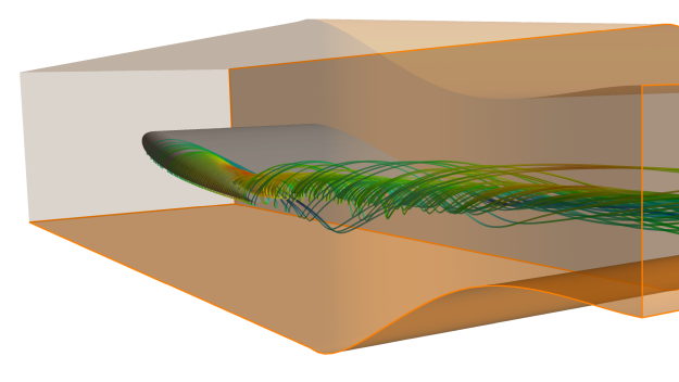
including velocity fields, pressure and Reynolds stresses. The 3D wing shown on Figure 12.111: NACA-0012 wing setup in a wind tunnel showing wing tip vortices as visualized by streamlines. has a rounded tip and is placed inside a wind tunnel. Due to the
lift, the flow from the pressure side travels around the rounded wing tip and rolls up into a
strong vortex downstream. The chord-based Reynolds number is  =4.6 million, the Mach number is approximately 0.1 and the angle of attack is
 . In the experiment, the flow is tripped at the leading edge so that the flow
can be considered as fully turbulent.
. In the experiment, the flow is tripped at the leading edge so that the flow
can be considered as fully turbulent.
Figure 12.111: NACA-0012 wing setup in a wind tunnel showing wing tip vortices as visualized by streamlines.
The following boundary conditions are adopted for the present simulations. At the inlet
section, a total pressure value of  = 1760 [Pa] above the atmospheric pressure is specified. Turbulent
characteristics at the inlet section are computed from the turbulent intensity value of
= 1760 [Pa] above the atmospheric pressure is specified. Turbulent
characteristics at the inlet section are computed from the turbulent intensity value of  = 0.15% and an eddy-to-molecular viscosity ratio equal to
  = 5. A mass flow
rate of
= 5. A mass flow
rate of  = 67.25 [kg/s] is imposed at the outlet boundary. This results in an area averaged
inlet velocity of
= 67.25 [kg/s] is imposed at the outlet boundary. This results in an area averaged
inlet velocity of  = 51.81 [m/s] matching the experimental value. The boundary layer on
the wind tunnel walls is not considered. Thus, symmetry boundary conditions are specified on
the wind tunnel walls for the slip wall imitation and no-slip condition is specified on the
NACA-0012 wing.
= 51.81 [m/s] matching the experimental value. The boundary layer on
the wind tunnel walls is not considered. Thus, symmetry boundary conditions are specified on
the wind tunnel walls for the slip wall imitation and no-slip condition is specified on the
NACA-0012 wing.
The mechanism of the curvature correction can be seen through the eddy-viscosity
distribution shown in Figure 12.112: Front view of eddy-viscosity ratio contours computed with the use of SST and SST-CC turbulence models downstream of the NACA-0012 wing [44]. for station  = 0.67 downstream of the trailing edge. The lower turbulent viscosity in the
vortex core region provided by the SST-CC model is a result of the reduction of production of
turbulent kinetic energy by the CC modification. This prevents a premature decay of the core
axial velocity to a value well below that found in the free-stream.
= 0.67 downstream of the trailing edge. The lower turbulent viscosity in the
vortex core region provided by the SST-CC model is a result of the reduction of production of
turbulent kinetic energy by the CC modification. This prevents a premature decay of the core
axial velocity to a value well below that found in the free-stream.
Figure 12.112: Front view of eddy-viscosity ratio contours computed with the use of SST and SST-CC turbulence models downstream of the NACA-0012 wing [44].
![Front view of eddy-viscosity ratio contours computed with the use of SST and SST-CC turbulence models downstream of the NACA-0012 wing [].](graphics/image093.png)
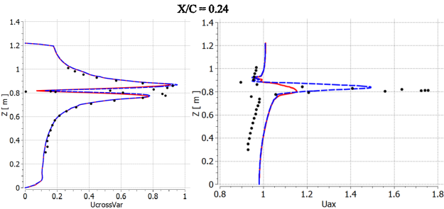
The predicted non-dimensional cross flow velocity and axial velocity at three planes
located downstream of the trailing edge are shown in Figure 12.113: Non-dimensional cross flow velocity (UcrossVar) and axial velocity (Uax) at three planes located downstream of the trailing edge of the NACA 0012 wing tip [44]. in
comparison with the experimental data. The coordinate  is based on the distance from the trailing edge. One can see that the vortex
strength is better captured by the SST-CC model as measured by the maximum of the streamwise
velocity. The original SST model provides too fast vortex decay, which is clear also through
the axial velocity plots. The SST-CC model shows a significant improvement at the station
is based on the distance from the trailing edge. One can see that the vortex
strength is better captured by the SST-CC model as measured by the maximum of the streamwise
velocity. The original SST model provides too fast vortex decay, which is clear also through
the axial velocity plots. The SST-CC model shows a significant improvement at the station
 = 0.24 when compared to SST. However, at the far downstream location,
 = 0.67, even the SST-CC model is no longer able to reproduce the experimental
velocity profiles, although though the eddy-viscosity is significantly reduced by the
correction. There is however also some mismatch in the axial freestream values which points to
a potential discrepancy between the experiments and the CFD set-up.
= 0.67, even the SST-CC model is no longer able to reproduce the experimental
velocity profiles, although though the eddy-viscosity is significantly reduced by the
correction. There is however also some mismatch in the axial freestream values which points to
a potential discrepancy between the experiments and the CFD set-up.
Figure 12.115: Computed distributions of the axial velocity at the plane passing through the vortex core for the NACA 0012 wing tip vortex [44]. Top view. shows the effect of the CC in a contour plot of the
axial velocity for a plane going through the vortex core. The increased region of flow
acceleration when using the CC extension is clearly visible. It breaks down however just
upstream of the  = 0.67 measurement station.
Figure 12.113: Non-dimensional cross flow velocity (UcrossVar) and axial velocity (Uax) at three planes located downstream of the trailing edge of the NACA 0012 wing tip [44].
![Non-dimensional cross flow velocity (UcrossVar) and axial velocity (Uax) at three planes located downstream of the trailing edge of the NACA 0012 wing tip [].](graphics/image094.5.png)
X/C=0.0
X/C=0.24
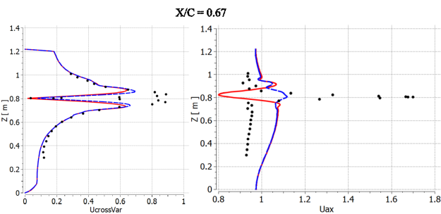
Figure 12.115: Computed distributions of the axial velocity at the plane passing through the vortex core for the NACA 0012 wing tip vortex [44]. Top view.
![Computed distributions of the axial velocity at the plane passing through the vortex core for the NACA 0012 wing tip vortex []. Top view.](graphics/image100.png)
The hydro-cyclone's typical flow structure and geometry is shown in Figure 12.116: Flow structure in the hydro-cyclone visualized by the streamlines.. The principle behind the cyclone separation is to utilize the strong radial force acting on particles in a strongly swirling flows. The fluid/particle mixture is injected tangentially into the cyclone and spirals downwards in the cyclone barrel (cylindrical section) and then in the cyclone conical section. Under the influence of centrifugal forces, the heavy particles are pushed towards the wall and exit the cyclone due to gravity at the lower exit. The light phase moves towards the cyclone axis, where it joins the upwards flow in a central vortex, leaving the cyclone through the upper outlet. Flow inside a hydro cyclone is characterized by the formation of a strong vortex core in the central region. To predict such flows accurately, the correct representation of the turbulence is a challenging task for turbulence models.
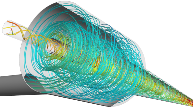
The current simulations are carried out for the hydro-cyclone investigated experimentally by Hartley [45]. Experimental data of axial and tangential velocities are available at various vertical locations in the cyclone. It is important to note that with a steady-state approach, no physically correct results are obtained, so the case is run in unsteady mode. This is physically correct as it is known that the vortex core is not stable and meanders around the axis of the cyclone.
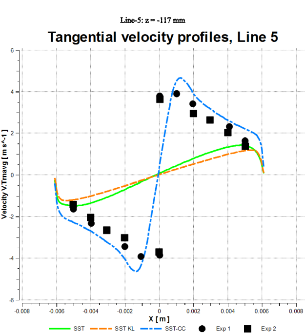
Figure 12.118: Time-averaged profiles of the tangential velocity in the hydro cyclone [45]. shows the sensitivity of the simulated tangential
velocity to the choice of turbulence model for various z-locations in the hydro-cyclone as
indicated in Figure 12.117: Measurement planes in the hydro cyclone [45].. The location z =  20 mm is just below the vortex finder. Here, the typical Rankine-vortex is
clearly visible from the experimental data, showing an 'inviscid' vortex at the outer radii and
a solid-body rotation close to the axis. The original SST model does not predict the 'inviscid'
vortex at large radii, with a tendency towards a solid body rotation everywhere. A substantial
improvement can be obtained by applying the curvature correction method for the SST model. The
main mechanism of the curvature correction lies in capturing the stabilizing effect of "solid
body rotation" near the axis which results in a strong reduction of the turbulence (and
therefore eddy-viscosity) in that region. In the comparison there is also the combination of
the SST model with the Kato-Launder production limiter (see Limiters) included. This modification does influence vortex flows as
vorticity and strain rate are no longer equal. However, the effect is small compared to the CC
modification.
20 mm is just below the vortex finder. Here, the typical Rankine-vortex is
clearly visible from the experimental data, showing an 'inviscid' vortex at the outer radii and
a solid-body rotation close to the axis. The original SST model does not predict the 'inviscid'
vortex at large radii, with a tendency towards a solid body rotation everywhere. A substantial
improvement can be obtained by applying the curvature correction method for the SST model. The
main mechanism of the curvature correction lies in capturing the stabilizing effect of "solid
body rotation" near the axis which results in a strong reduction of the turbulence (and
therefore eddy-viscosity) in that region. In the comparison there is also the combination of
the SST model with the Kato-Launder production limiter (see Limiters) included. This modification does influence vortex flows as
vorticity and strain rate are no longer equal. However, the effect is small compared to the CC
modification.
![Measurement planes in the hydro cyclone [].](graphics/afterimage2.png)
![Time-averaged profiles of the tangential velocity in the hydro cyclone [].](graphics/image103.5.png)
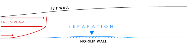
The primary focus of the NASA Hump Flow [46]–[48] (Figure 12.119: Schematic of the NASA hump flow.) is to assess the ability of turbulence models to predict 2-D separation from a smooth body (caused by an adverse pressure gradient) as well as the subsequent reattachment and boundary layer recovery. Since its introduction, this case has proved to be a challenge for all known RANS models.
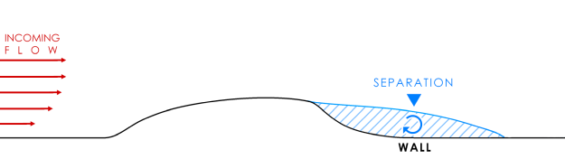
Models tend to underpredict the turbulent shear-stress and the turbulent kinetic energy in the separated shear layer, and therefore tend to predict too long a separation bubble. This is an issue with all RANS models and is one the main remaining deficiencies of this model family. It is important to note that the effect is not observed for cases where the separation is fixed by the geometry, like in a backward facing step (see Figure 12.61: Wall shear stress coefficient, Cf (left) and wall heat transfer coefficient, St, (right) for backward-facing step flow (12).). It seems that the difference between these cases lies in a potential unsteadiness of the separation line for the hump flow, which could result in small-scale vortex shedding. Such an effect is in principle outside the realm of RANS models, as it constitutes unsteady flow and not turbulence. Naturally, there is a desire to model such effects within the existing RANS models, as the alternative would be much more expensive Scale-Resolving Simulations. For this reason, different, highly ad-hoc RANS model enhancements have been proposed. They are not used widely and should not generally be activated. However, in some applications, they have shown some improvements and one of the methods is therefore discussed here. The model presented is implemented in Ansys CFX. The formulation has also been adopted in a NASA TM by Rumsey [49] using different coefficients.
As the SST model typically predicts the onset of separation with good accuracy, there is a
need to introduce additional production of turbulence under such conditions. The Reattachment
Modification (RM) model introduces the production term  into the SST model to enhance
turbulence levels in the separating shear layers emanating from walls.
into the SST model to enhance
turbulence levels in the separating shear layers emanating from walls.
 | (12–41) |
The motivation for this formulation is that in the separating shear layer, the ratio
 increases significantly beyond one, which can then be used as an indicator to
trigger the additional production term. Unfortunately, the reattachment modification is very
sensitive to the combination of the computational mesh resolution and numerics for the
turbulence equations. Three meshes as shown in Figure 12.120: Computational meshes for the Hump flow. have been
tested, with Mesh-1 being the finest and Mesh-3 the coarsest. Figure 12.121: Comparison of wall shear stress coefficient for NASA Hump flow.
shows the effect of the RM on the solution, as a function of mesh and discretization. The RM
improves the prediction of the reattachment point only on the coarse meshes (Mesh-3) for the
first order upwind scheme. The results of the original SST model and the SST-RM model using 2nd
order numerics are virtually the same for all the meshes. The efficiency of the model can be
improved by reducing the limiter of 1.6 in the equation, but this can have the effect that the
modification will affect generic flows, especially turbulent mixing layers. The spreading rate
of mixing layers would then be over-predicted. The NASA version of the model effectively reduces
the limiter from 1.6
increases significantly beyond one, which can then be used as an indicator to
trigger the additional production term. Unfortunately, the reattachment modification is very
sensitive to the combination of the computational mesh resolution and numerics for the
turbulence equations. Three meshes as shown in Figure 12.120: Computational meshes for the Hump flow. have been
tested, with Mesh-1 being the finest and Mesh-3 the coarsest. Figure 12.121: Comparison of wall shear stress coefficient for NASA Hump flow.
shows the effect of the RM on the solution, as a function of mesh and discretization. The RM
improves the prediction of the reattachment point only on the coarse meshes (Mesh-3) for the
first order upwind scheme. The results of the original SST model and the SST-RM model using 2nd
order numerics are virtually the same for all the meshes. The efficiency of the model can be
improved by reducing the limiter of 1.6 in the equation, but this can have the effect that the
modification will affect generic flows, especially turbulent mixing layers. The spreading rate
of mixing layers would then be over-predicted. The NASA version of the model effectively reduces
the limiter from 1.6 1.25 resulting in a more active model, but at the price of affecting generic
flows.
1.25 resulting in a more active model, but at the price of affecting generic
flows.
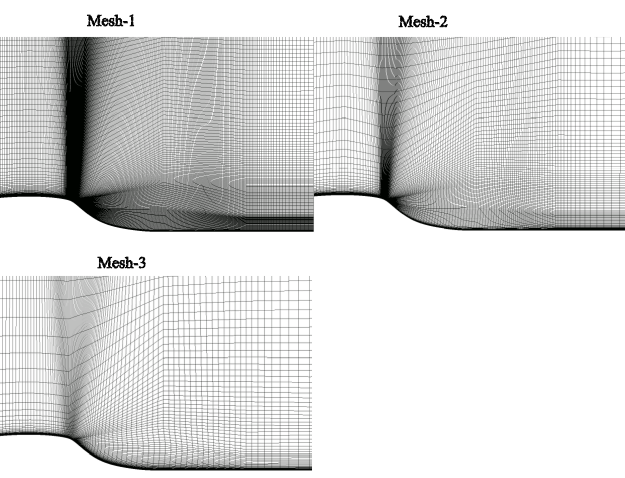
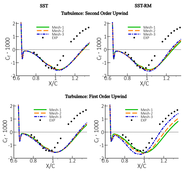
An improvement of the reattachment prediction can also be achieved with the turning of the
GEKO model. Figure 12.122: Comparison of wall shear stress coefficient predicted with GEKO model for NASA Hump flow [48]. shows the effect of the decrease of the
 coefficient on the prediction of the reattachment point. The prediction of the
velocity and Reynolds stresses are also improved for the
coefficient on the prediction of the reattachment point. The prediction of the
velocity and Reynolds stresses are also improved for the  = 1.00 value (Figure 12.123: Effect of the GEKO CSEP on the streamwise velocity for NASA Hump flow [46], [47].) albeit at the expense of
delayed separation onset prediction. However, the Reynolds normal stresses
= 1.00 value (Figure 12.123: Effect of the GEKO CSEP on the streamwise velocity for NASA Hump flow [46], [47].) albeit at the expense of
delayed separation onset prediction. However, the Reynolds normal stresses  are still underpredicted in the separation region and virtually independent of
the
are still underpredicted in the separation region and virtually independent of
the  value which is shown in Figure 12.124: Effect of the GEKO CSEP on the Reynolds shear stresses for NASA Hump flow [46], [47]..
Figure 12.122: Comparison of wall shear stress coefficient predicted with GEKO model for NASA Hump flow [48].
![Comparison of wall shear stress coefficient predicted with GEKO model for NASA Hump flow [].](graphics/image121.5.png)
![Effect of the GEKO CSEP on the streamwise velocity for NASA Hump flow [], [].](graphics/image123.png)
Figure 12.124: Effect of the GEKO CSEP on the Reynolds shear stresses for NASA Hump flow [46], [47].
![Effect of the GEKO CSEP on the Reynolds shear stresses for NASA Hump flow [], [].](graphics/image124.png)
Again, it needs to be stressed that the change to  =1.00 is not considered a model for
the true physics of these flows, but can help in practical applications to obtain better
agreement with the data.
=1.00 is not considered a model for
the true physics of these flows, but can help in practical applications to obtain better
agreement with the data.
Impinging jets are a very effective way to enhance surface heat transfer and are frequently employed in industrial devices (impingement cooling). The considered test case is based on the experiments carried out by Baughn et al. [50]. The flow being modeled is the incompressible flow of a turbulent jet impinging onto a flat plate. Figure 12.125: Scheme of the impinging jet flow shows the geometry of the flow domain. The size of the computational domain in the plane is 13D by 13D, where D = 0.0265 [m] is the diameter of the pipe.
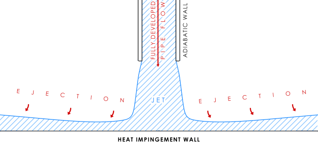
The computational domain with boundary conditions is shown in Figure 12.126: Computational domain with boundary conditions and mesh for the impinging jet.. The inflow conditions for velocity and turbulence are specified
using profiles for fully developed turbulent flow through a pipe, which are calculated in
separate simulations. The Reynolds number based on the bulk inlet velocity,  = 15.45 [m/s], and pipe diameter is Re =
  . The heated surface is modeled as a wall with a specified constant heat flux,
 = 300 [W/m]. All other walls are treated as adiabatic walls. An auxiliary inlet
boundary condition is employed to allow for entrainment of fluid from outside. Zero gauge total
pressure along with the inflow direction is assumed on this segment. The right boundary is
modeled as a modified outlet boundary which changes to an inlet with 10 degrees flow direction
to the boundary, in case fluid enters the domain. This treatment avoids massive flow entrainment
at that boundary.
= 300 [W/m]. All other walls are treated as adiabatic walls. An auxiliary inlet
boundary condition is employed to allow for entrainment of fluid from outside. Zero gauge total
pressure along with the inflow direction is assumed on this segment. The right boundary is
modeled as a modified outlet boundary which changes to an inlet with 10 degrees flow direction
to the boundary, in case fluid enters the domain. This treatment avoids massive flow entrainment
at that boundary.
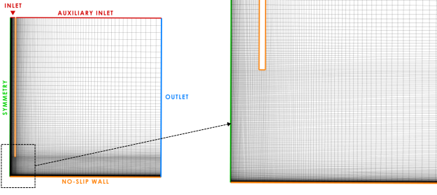
Figure 12.127: Local Nusselt number computed using different turbulence models (left) and SST model with and without taking into accout the laminar turbulent transition (right).(left) compares the predicted Nusselt number
distributions for different turbulence models. The  and SA models underestimate Nu over almost the entire length of the heated
wall, while the SST model gives a reasonable agreement downstream from
and SA models underestimate Nu over almost the entire length of the heated
wall, while the SST model gives a reasonable agreement downstream from  = 1.5. However, all the models fail in predicting the dip in the Nu number at
 < 1.5. To investigate this further, a simulation is performed, where the
SST model is combined with the
< 1.5. To investigate this further, a simulation is performed, where the
SST model is combined with the  -transition model (36). Figure 12.127: Local Nusselt number computed using different turbulence models (left) and SST model with and without taking into accout the laminar turbulent transition (right). (right) demonstrates
that the inclusion of the laminar-turbulent transition phenomena is essential in predicting the
local minima. It coincides with the location of laminar-turbulent transition of the boundary
layer developing on the impingement wall, which is triggered by the shear layer from the outer
boundary of the impinging jet. Note that in case of the transition computations, the
computational mesh (see Figure 12.128: Computational mesh for the fully turbulent regime (left) and regime with taking into account laminar-turbulent transition (Right).) was refined in radial direction
(
-transition model (36). Figure 12.127: Local Nusselt number computed using different turbulence models (left) and SST model with and without taking into accout the laminar turbulent transition (right). (right) demonstrates
that the inclusion of the laminar-turbulent transition phenomena is essential in predicting the
local minima. It coincides with the location of laminar-turbulent transition of the boundary
layer developing on the impingement wall, which is triggered by the shear layer from the outer
boundary of the impinging jet. Note that in case of the transition computations, the
computational mesh (see Figure 12.128: Computational mesh for the fully turbulent regime (left) and regime with taking into account laminar-turbulent transition (Right).) was refined in radial direction
( 1.5) for the proper resolution of the laminar-turbulent transition zone (this
refinement had no effect on the fully turbulent simulations).
1.5) for the proper resolution of the laminar-turbulent transition zone (this
refinement had no effect on the fully turbulent simulations).
Figure 12.127: Local Nusselt number computed using different turbulence models (left) and SST model with and without taking into accout the laminar turbulent transition (right).
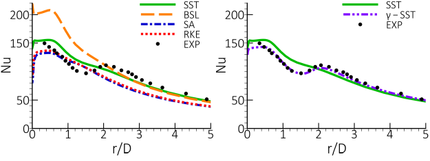
Figure 12.128: Computational mesh for the fully turbulent regime (left) and regime with taking into account laminar-turbulent transition (Right).
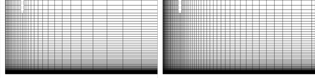
The following topics are discussed:
A stably-stratified mixing layer flow between fresh water and saline stream was experimentally investigated by Uittenbogaard [51] at the Delft Hydraulics laboratory. Their installation is sketched in Figure 12.129: Scheme of the stratified mixing layer. Two flows with different densities enter the domain horizontally separated by a splitter plate. The upper flow is a fresh water stream with a density of 1015 [kg/m3] and an average velocity of 0.52 [m/s]. The lower current is a salt water solution with density of 1030 [kg/m3] and an average velocity of 0.32 [m/s]. The flow can be considered two dimensional in the CFD setup as shown in Figure 12.129: Scheme of the stratified mixing layer. The flow properties are presented in Table 3.
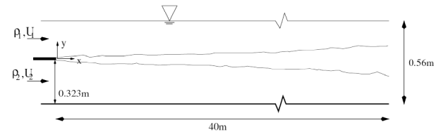
Figure 68: Scheme of the stratified mixing layer.
Table 12.12: Flow parameters of the stratified mixing layer
kg/ |
kg/ |
Pa s | Thermal Conductivity, W/(m K) | Mass Diffusivity,
| Specific Heat, J/(Kg K) | Molecular Weight, kg/kmol |
|---|---|---|---|---|---|---|
1015 | 1030 |
| 0.6069 |
| 4182 | 18.0152 |


The computational domain with boundary conditions is shown in Figure 12.130: Computational domain with boundary conditions and mesh for the stratified mixing layer.. The length and height of domain are 40 [m] and 0.56 [m] corresponding to the experimental test section. At the inlet boundary, the thickness of the fresh/salt water layer is 0.237 and 0.323 [m] respectively.
Computations are carried out with Standard  model and SST and GEKO models
without and with buoyancy corrections. For all the cases, the boundary conditions are as follows. At the inlet boundary, the
experimental velocity profiles, turbulence characteristics and component concentration are
specified. Constant pressure is specified on the outlet boundary. The lower boundary is modeled
as the non-slip wall and upper boundary of the flow is a free surface.
model and SST and GEKO models
without and with buoyancy corrections. For all the cases, the boundary conditions are as follows. At the inlet boundary, the
experimental velocity profiles, turbulence characteristics and component concentration are
specified. Constant pressure is specified on the outlet boundary. The lower boundary is modeled
as the non-slip wall and upper boundary of the flow is a free surface.
Figure 12.130: Computational domain with boundary conditions and mesh for the stratified mixing layer.
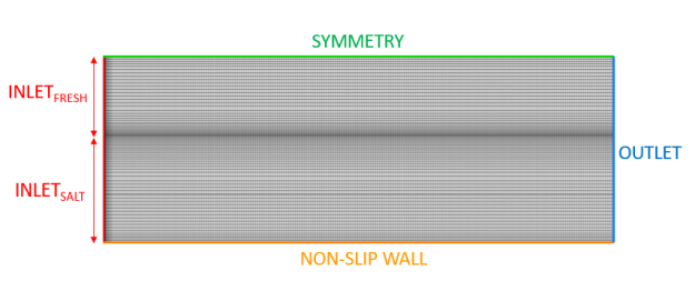
Figure 70 shows comparison of the density and velocity profiles at three different
sections for the SST model without and with buoyancy correction (SST-BC).  = 5 [m] is the section near the inlet boundary and
  = 40 [m] corresponds to the outlet location. The non-dimensional density
variable computes as
= 40 [m] corresponds to the outlet location. The non-dimensional density
variable computes as  . It is evident from Figure 12.133: Density field for the SST (Left) and SST-BC (Right) model. that without
considering buoyancy effects the stabilizing effect of the density stratification is not felt
and the rate of mixing of the two fields is excessive. The buoyancy production terms reduce the
turbulence kinetic energy generated in the shear layer as shown in Figure 12.134: Turbulence kinetic energy field for the SST (Left) and SST-BC (Right) model.. It leads to a reduction of the eddy viscosity and the Reynolds
shear stresses. As a result, the mixing layer develops in better agreement with the experiment.
The station furthest downstream at
. It is evident from Figure 12.133: Density field for the SST (Left) and SST-BC (Right) model. that without
considering buoyancy effects the stabilizing effect of the density stratification is not felt
and the rate of mixing of the two fields is excessive. The buoyancy production terms reduce the
turbulence kinetic energy generated in the shear layer as shown in Figure 12.134: Turbulence kinetic energy field for the SST (Left) and SST-BC (Right) model.. It leads to a reduction of the eddy viscosity and the Reynolds
shear stresses. As a result, the mixing layer develops in better agreement with the experiment.
The station furthest downstream at  =40[m] indicates that the buoyancy correction imposes too strong a damping
effect on turbulence as seen by the lack of mixing in both the density and the velocity
profiles. Default settings were used and no effort was undertaken to fine-tune the model.
=40[m] indicates that the buoyancy correction imposes too strong a damping
effect on turbulence as seen by the lack of mixing in both the density and the velocity
profiles. Default settings were used and no effort was undertaken to fine-tune the model.
Figure 12.131: Density and streamwise velocity profiles at different sections for the stratified mixing layer.
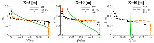
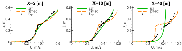
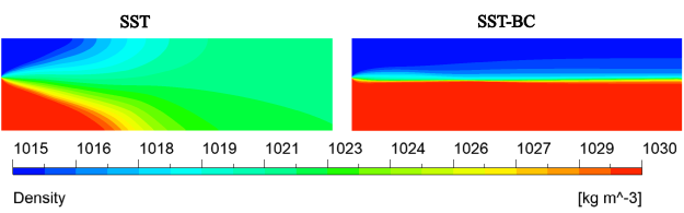
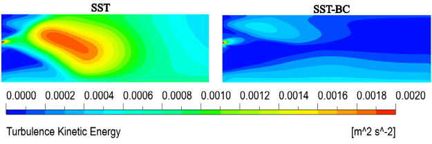
The comparison of different turbulence models shown in Figure 12.135: Density (upper row) and streamwise velocity (lower row) profiles for diferent models for the stratified mixing layer at X = 10 [m] section.
demonstrates that the sensitivity to the turbulence model is negligible and much smaller than
the buoyancy effects. Due to similar results for different sections only  = 10 [m] is shown.
Figure 12.135: Density (upper row) and streamwise velocity (lower row) profiles for diferent models for the stratified mixing layer at X = 10 [m] section.
![Density (upper row) and streamwise velocity (lower row) profiles for diferent models for the stratified mixing layer at X = 10 [m] section.](graphics/image149.5.png)
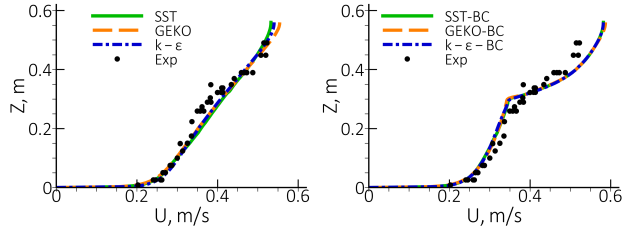
As mentioned in section 3.3.5 the use of limiters in the formulation of the eddy-viscosity
or the production term prevents the formation of unphysically high turbulent kinetic energy
levels and, therefore, high eddy-viscosity levels near stagnation regions. It should be noted
that the unphysical build-up of turbulence does not only occur in stagnation regions, but in any
other region with non-zero shear strain rate,  , outside shear layers (e.g. also in accelerating
inviscid flow).
, outside shear layers (e.g. also in accelerating
inviscid flow).
Detailed descriptions of the limiters are given in Limiters. This section demonstrates the effect of realizability limiters, the production limiter and
the Kato-Launder limiter for different turbulence models for flow around a NACA-4412 airfoil at
 . Note that RKE model features an internal realizability limiter which cannot be turned
off. This limiter is not the same as the realizability limiter used in the GEKO model. As shown
below, it is also not as effective as the GEKO limiter.
. Note that RKE model features an internal realizability limiter which cannot be turned
off. This limiter is not the same as the realizability limiter used in the GEKO model. As shown
below, it is also not as effective as the GEKO limiter.
For all the Figures the following notation is used:
 – Realizibility limiter (Eq (9.34))
 – Production term limiter (Eq (9.53))
 – Kauto-Launder production term formulation (Eq (9.52))
As seen in Figure 12.136: Effect of limiters for the GEKO model near the stagnation point for flow around airfoils Figure 74, Figure 12.137: Effect of production limiter for the  Standard model near the stagnation point for flow around airfoils.
Figure 75 and Figure 12.138: Eddy-viscosity field predicted with the RKE turbulence model near the stagnation region for flow around airfoils., all the considered limiters avoid the
eddy-viscosity and turbulent kinetic energy build-up in the stagnation regions of a NACA 4412
airfoil. For the GEKO model, the default
Standard model near the stagnation point for flow around airfoils.
Figure 75 and Figure 12.138: Eddy-viscosity field predicted with the RKE turbulence model near the stagnation region for flow around airfoils., all the considered limiters avoid the
eddy-viscosity and turbulent kinetic energy build-up in the stagnation regions of a NACA 4412
airfoil. For the GEKO model, the default  has the same effect as other limiters. The effect of the production limiter is
strongest for the
has the same effect as other limiters. The effect of the production limiter is
strongest for the  Standard model. On the other hand, the in-built realizability limiter of the
 RKE model improves the solution in the stagnation region, however, the model
still predicts high eddy-viscosities outside the boundary layer. Again, the use of the
RKE model improves the solution in the stagnation region, however, the model
still predicts high eddy-viscosities outside the boundary layer. Again, the use of the
 fixes this issue.
In case of laminar-turbulent transition modeling, the effectiveness of limiters is very important, even small turbulence build-up can affect the transition onset location. Typically, a strong combination of limiters is used (Pk limiter and Kato-Launder for the SST model).
Figure 12.136: Effect of limiters for the GEKO model near the stagnation point for flow around airfoils
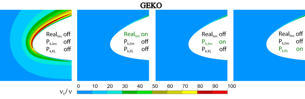
Figure 12.137: Effect of production limiter for the Standard model near the stagnation point for flow around airfoils.
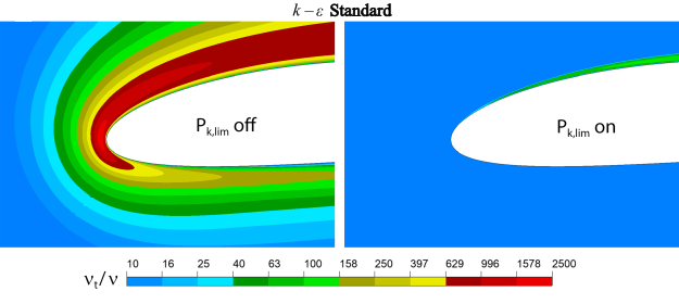
Figure 12.138: Eddy-viscosity field predicted with the RKE turbulence model near the stagnation region for flow around airfoils.
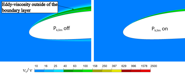
Mesh resolution and mesh quality are key elements for a successful CFD simulation. There are several nested requirements for mesh resolution:
The following topics are discussed:
The most basic requirement is that the grid must be able to resolve the inviscid parts of the flow. This means that regions of flow acceleration/deceleration as well as streamline curvature etc. must be properly resolved. This also includes the resolution of strong gradients, especially shocks. Inviscid flow resolution is typically of importance in regions of geometrical changes (corners, edges, trailing edges, leading edge suction peaks, inviscid vortex flows, ….). Insufficient mesh resolution in this context is typically noticeable through changes in pressure distribution under mesh refinement.
Free shear flows, like mixing layers, jets or wakes typically require at least ~10 cells normal to the layer. The resolution in stream/spanwise direction is usually of the order of the shear layer thickness.
There are two main challenges with free shear layers. The first is that they can be very thin at their origin. It is therefore hard to capture the initial formation of such layers – in most cases they are therefore under-resolved. The second challenge is that their location is often not known before the simulation. One should therefore investigate the solutions and refine the meshes if important shear layers have been missed or under-resolved by the mesh. Alternatively, the layers can be targeted by mesh adaptation using adaptation criteria indicative of the layer (gradients of velocity or turbulent kinetic energy etc.).
Figure 12.139: Computational meshes for the mixing layer. shows examples of coarse, medium and fine meshes which correspondingly have ~ 5/10/20 cells across the mixing layer. For all the meshes the streamwise resolution is identical. The coarse mesh does not provide the grid-independent solution while results on the medium and fine meshes are in perfect agreement. This is shown on Figure 12.140: Comparison of the velocity (left), turbulence kinetic energy (middle) and Reynolds shear-stress (right) profiles on different meshes for the mixing layer. where self-similar profiles of the streamwise velocity component, turbulence kinetic energy and Reynolds shear stress are plotted for the SST model.
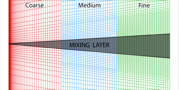
Figure 12.140: Comparison of the velocity (left), turbulence kinetic energy (middle) and Reynolds shear-stress (right) profiles on different meshes for the mixing layer.
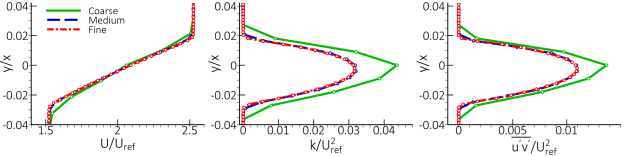
Wall boundary layers are the most demanding in terms of mesh resolution, as the solution
gradients inside boundary layers can be very high. This is true for both, primary solution
variables, like velocity or temperature, but even more so for turbulence quantities like  ,
,  ?
or
?
or  .
.
Most CFD users are fixated on the  values of the first cell center of the wall cells and assume that achieving a
given threshold
values of the first cell center of the wall cells and assume that achieving a
given threshold  value ensures enough mesh resolution inside the boundary layer. This is not
the case as a given
value ensures enough mesh resolution inside the boundary layer. This is not
the case as a given  value does not by itself ensure that there are enough cells inside the
boundary layer. It is important to understand that for the same
value does not by itself ensure that there are enough cells inside the
boundary layer. It is important to understand that for the same  -value and the same grid expansion ratio (growth rate between cells

there would be many more cells inside a high Reynolds number boundary layer
than in a low Reynolds number one. This is clear from Figure 12.141: Boundary layer thickness in wall units for low and high Reynolds number. which
shows that the boundary layer thickness in terms of  is much larger for the high than for the low Reynolds number case.
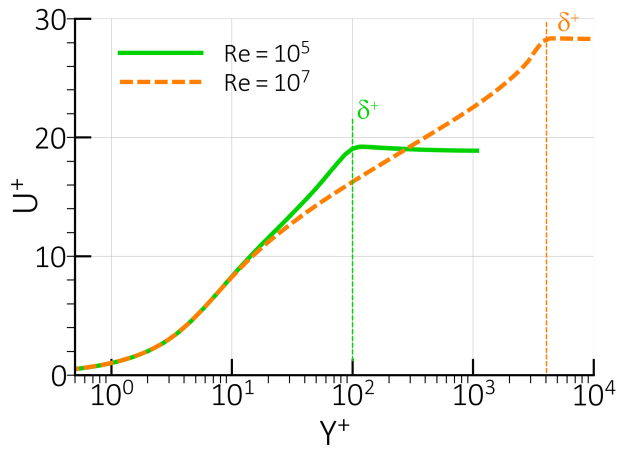
The main quality criterion for boundary layer meshes is therefore not  , but the number of cells (prism layers) inside the boundary layer (estimates
of boundary layer thickness are given in Section 9.4). It is important to stress the word
'inside', as prism layers generated with a given number of cells do not ensure that the layers
are resolving the boundary layer – it is easy to create prism layers where the boundary
layer is much thinner or much thicker than the prism layer height. If prismatic layers cover
only a part of the boundary layer (see Figure 12.142: Computational unstructured mesh with prismatic layers (red) thinner than the boundary layer (blue line) thickness.) it is under-resolved
due to a large edge length change from the prism layers to the tetra/poly cells. In this case,
the outer part of the boundary layer cannot be resolved.
, but the number of cells (prism layers) inside the boundary layer (estimates
of boundary layer thickness are given in Section 9.4). It is important to stress the word
'inside', as prism layers generated with a given number of cells do not ensure that the layers
are resolving the boundary layer – it is easy to create prism layers where the boundary
layer is much thinner or much thicker than the prism layer height. If prismatic layers cover
only a part of the boundary layer (see Figure 12.142: Computational unstructured mesh with prismatic layers (red) thinner than the boundary layer (blue line) thickness.) it is under-resolved
due to a large edge length change from the prism layers to the tetra/poly cells. In this case,
the outer part of the boundary layer cannot be resolved.
Figure 12.142: Computational unstructured mesh with prismatic layers (red) thinner than the boundary layer (blue line) thickness.
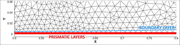
There is no single number of how many cells across a boundary layer are optimal, as this depends on the type of flow and the required accuracy. The highest accuracy demands are for external aeronautical applications with safety concerns – especially aircraft simulations. For such flows, boundary layers are often resolved with 30-40 cells. For most industrial flows, 10 layers inside the boundary layer are reasonable. However, there are also many technical flows, where only smaller cell counts can be afforded, and reasonable solutions can often be achieved with only 3-5 layers.
The need to accurately resolve the boundary layer increases with the need:
To resolve flow separation from smooth surfaces like airfoils (contrary to separation from geometric discontinuities like edge or corners).
Flows with heat transfer, where the resolution of conditions in the very near wall region is important. This is even more important for flows with high Prandtl numbers where the thermal sublayer is very thin.
Flows with laminar-turbulent transition where the laminar boundary layers are typically very thin and needs to be resolved for the transition model to operate properly (see below).
Streamwise resolution is typically several times the boundary layer thickness (say1-5) whereas 'spanwise' grid spacing can be even higher depending on the gradients in that direction (for 2D flows it can be arbitrarily coarse). However, in most technical flows, there is no clear distinction between streamwise and spanwise and the grid surface spacing is then typically selected as 'isotropic'.
Grid resolution of boundary layers should be checked during and/or after the simulation. A
good quantity to visualize is the ratio of turbulent to molecular viscosity ( ). It has a maximum near the center of the boundary layer and decays to low
freestream values outside the layer. Visualizing TVR in a contour plot with overset grid lines
allows a good estimate of grid resolution by counting the wall normal cells which are inside
the elevated TVR levels near the wall. This is shown in Figure 12.143: The boundary layers thickness visualized by eddy-viscosity ratio field for different meshes around NACA-4412 airfoil. Blue color shows the area of the inviscid flow. for
different grids for a NACA 4412 airfoil. Here the fine grid provides a grid-independent
solution while the boundary layer is under resolved near the leading edge for the coarse and
medium grids. There are ~ 5 cells across the boundary layer near the leading edge for the
medium mesh and the coarse mesh does not resolve the boundary layer at all. As a result, the
boundary layer is thicker for these meshes which leads to earlier separation (see Figure 12.145: Comparison of velocity profiles on different meshes for flow around the NACA-4412 airfoil.) on the suction side of the airfoil. The local mesh refinement in
wall normal direction in the leading edge region shown in Figure 12.146: Local mesh refinement on the leading edge for the medium mesh.
improves the prediction of the boundary layer. Figure 12.147: Comparison of the velocity profiles on the medium and refined medium (medium+LE) meshes. shows that
the results on the refined medium mesh and on the fine mesh are in good agreement.
). It has a maximum near the center of the boundary layer and decays to low
freestream values outside the layer. Visualizing TVR in a contour plot with overset grid lines
allows a good estimate of grid resolution by counting the wall normal cells which are inside
the elevated TVR levels near the wall. This is shown in Figure 12.143: The boundary layers thickness visualized by eddy-viscosity ratio field for different meshes around NACA-4412 airfoil. Blue color shows the area of the inviscid flow. for
different grids for a NACA 4412 airfoil. Here the fine grid provides a grid-independent
solution while the boundary layer is under resolved near the leading edge for the coarse and
medium grids. There are ~ 5 cells across the boundary layer near the leading edge for the
medium mesh and the coarse mesh does not resolve the boundary layer at all. As a result, the
boundary layer is thicker for these meshes which leads to earlier separation (see Figure 12.145: Comparison of velocity profiles on different meshes for flow around the NACA-4412 airfoil.) on the suction side of the airfoil. The local mesh refinement in
wall normal direction in the leading edge region shown in Figure 12.146: Local mesh refinement on the leading edge for the medium mesh.
improves the prediction of the boundary layer. Figure 12.147: Comparison of the velocity profiles on the medium and refined medium (medium+LE) meshes. shows that
the results on the refined medium mesh and on the fine mesh are in good agreement.
Coarse
Figure 12.143: The boundary layers thickness visualized by eddy-viscosity ratio field for different meshes around NACA-4412 airfoil. Blue color shows the area of the inviscid flow.
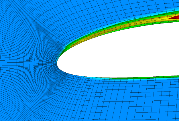
Medium
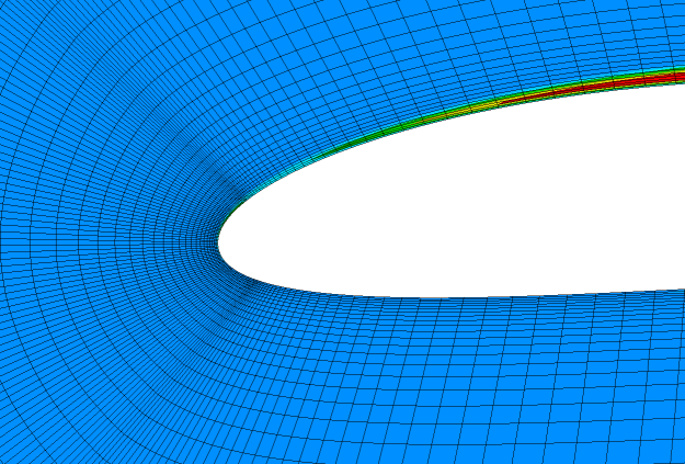
Fine
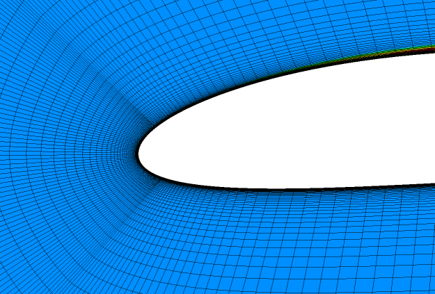
Figure 12.145: Comparison of velocity profiles on different meshes for flow around the NACA-4412 airfoil.
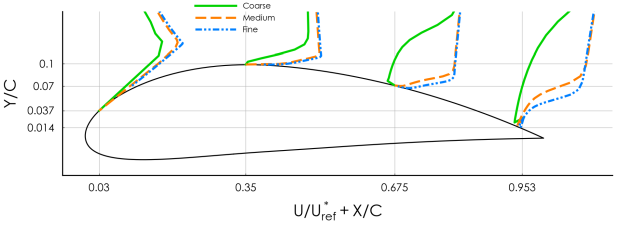
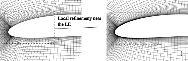
Figure 12.147: Comparison of the velocity profiles on the medium and refined medium (medium+LE) meshes.
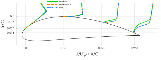
Another grid-quality measure is the smoothness by which prism layers merge into the outer unstructured mesh. Grids with large size jumps in this region should be avoided as they can inhibit the proper growth of the boundary layer (which then cannot grow outside the prism layer mesh due to low resolution). The optimal mesh structure:
Prismatic layers cover the entire boundary layer
The number of prismatic layers should be sufficient for the boundary layer resolution.
The first near wall grid step ensures
 <1 without wall treatment.
However, higher
 values can also be applied if the overall number of cells across
the layer is sufficient.
values can also be applied if the overall number of cells across
the layer is sufficient.
Smooth connection of the prismatic layers and tetra/poly cells.
Streamwise grid step at the wall should be sufficient for the proper resolution of the flow features.
stagnation region
separation
shock wave
transition
corner flow
Figure 12.148: Optimal unstructured mesh topology for flow around airfoil. illustrates the optimal mesh topology and resolution for an unstructured mesh for the flow around an airfoil.
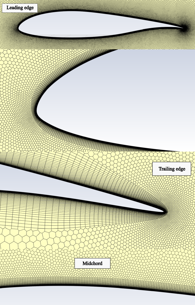
Boundary layers undergoing transition are more sensitive to the mesh resolution than fully turbulent boundary layer. Meshes for fully turbulent simulations are not sufficient in the transition region especially in the streamwise direction. Unfortunately, the transition location is unknown without precursor simulations in most cases. Therefore, a two-stage approach is recommended for the computations using transition models:
1st stage – computations on the baseline fine fully turbulent mesh and estimation of the transition region.
2nd stage – mesh refinement in streamwise, wall-normal and spanwise (in case of the fully three dimensional flow) directions in the transition region. Repeat until grid-converged solution is achieved.
It should be noted that the mesh requirements also depend on the transition model choice.
Here the three transition models described in section 3.4.1 are considered. Figure 12.150: Effect of the resolution of transition region in streamwise direction for different transition models for the T3A flat plate boundary layer. shows the effect of streamwise mesh resolution on the transition
prediction on the flat plate for different transition models. The baseline fully turbulent mesh
with streamwise grid step  (
( is boundary layer thickness) is only sufficient for the
  model but not for the other two models and should be refined in the
transition region. The baseline and refined meshes are shown on Figure 12.149: Computational meshes for the fully turbulent (upper) and transitional (lower) boundary layer.. For the refined mesh, the streamwise grid step is
model but not for the other two models and should be refined in the
transition region. The baseline and refined meshes are shown on Figure 12.149: Computational meshes for the fully turbulent (upper) and transitional (lower) boundary layer.. For the refined mesh, the streamwise grid step is  in the transition region and
  in the laminar and fully turbulent parts. In this context it is important to
note that for many technical devices, transition is triggered through laminar-turbulent bubble
separation. In such cases, the streamwise mesh resolution is even more important in order to
detect and resolve the laminar bubble. It is usually required to resolve the bubble with 5-10
streamwise cells. For this reason, it is not recommended in general to use coarse
in the laminar and fully turbulent parts. In this context it is important to
note that for many technical devices, transition is triggered through laminar-turbulent bubble
separation. In such cases, the streamwise mesh resolution is even more important in order to
detect and resolve the laminar bubble. It is usually required to resolve the bubble with 5-10
streamwise cells. For this reason, it is not recommended in general to use coarse
 spacings in transition simulations, as the mechanism of transition is often
not known a priori.
spacings in transition simulations, as the mechanism of transition is often
not known a priori.
In case of first near wall height variation the transition location is insensitive to
 <1 in the transition region (see Figure 12.151: Effect of the resolution of transition region in wall-normal wall direction for different transition models for T3A the flat plate boundary layer.). For
higher values of
<1 in the transition region (see Figure 12.151: Effect of the resolution of transition region in wall-normal wall direction for different transition models for T3A the flat plate boundary layer.). For
higher values of  in this area, the transition location moves upstream. For both streamwise and
wall-normal mesh studies the two-equation model (
in this area, the transition location moves upstream. For both streamwise and
wall-normal mesh studies the two-equation model ( ) is much less sensitive to the mesh resolution than one-equation
intermittency transition model (
) is much less sensitive to the mesh resolution than one-equation
intermittency transition model ( ), or the algebraic intermittency model (
 ), which is most sensitive to the mesh resolution.
Finally the basic recommendation for all the transition models for the mesh generation.
 in the transition region
 in the transition region
 in the transition region (
 )
)
Figure 12.149: Computational meshes for the fully turbulent (upper) and transitional (lower) boundary layer.
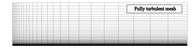
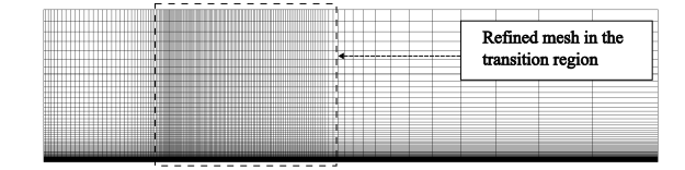
Figure 12.150: Effect of the resolution of transition region in streamwise direction for different transition models for the T3A flat plate boundary layer.
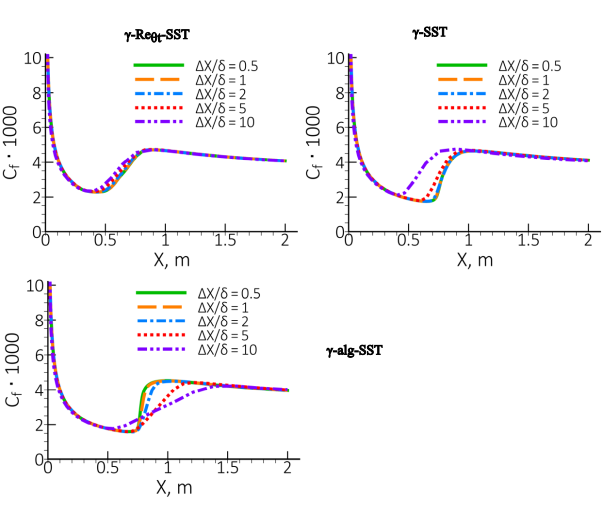
Figure 12.151: Effect of the resolution of transition region in wall-normal wall direction for different transition models for T3A the flat plate boundary layer.
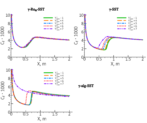
When activating the Corner Flow Correction or an EARSM to compute the secondary flow into corners, the mesh resolution into the corners especially for unstructured meshes (tetrahedral, polyhedral or cartesian) is critical.
Ideal meshes for corner flows are structured meshes as shown in Figure 12.152: Baseline structured mesh with fine resolution in the corners for the DLR-Diffuser [41]. where the wall normal refinement for one wall ensures automatically proper refinement into the corner for the adjacent walls (meaning small edge length on the wall going into the corner). Such corner mesh refinement avoids additional mesh refinement in streamwise direction which should be done for the unstructured meshes.
The meshing requirements to resolve the corner flow are especially challenging for the DLR diffuser (41) described in Section 4.3.2. For this test case, a uniform flow (U=10m/s, Tu=1%, TVR=1) was specified at the inlet. This results in a very thin boundary layer at the onset of the diffuser. While this boundary layer can easily be resolved in wall normal direction, it is much harder to resolve the flow dynamics into the corner (the secondary flow is taking place inside the boundary layer and has to be resolved in the plane normal to the mean flow direction). While the structured mesh (Str mesh) in Figure 12.152: Baseline structured mesh with fine resolution in the corners for the DLR-Diffuser [41]. has sufficient resolution in that area due to its mesh topology, the resolution of this zone by unstructured meshes is much harder. Two unstructured meshes, one without refinement (PH-1) and one with refinement (PH-2) into the corner are shown in Figure 12.153: Baseline mesh PH-1 (left) and refinement mesh PH-2 (right) near the corners for the unstructured meshes for the DLR-diffuser [41]. and Figure 12.154: Cross section of typical unstructured mesh PH-1 in rectangle channel (left) and collapsing of the prismatic cells near the corners on the refined mesh PH-2 (right) for the DLR-Diffuser [41].. Figure 12.155: Eddy viscosity of the developing boundary layer at the straight part of diffuser and mesh cross section mesh resolution for different meshes. shows contours of the eddy-viscosity ratio with the mesh plotted on top. It is intuitively clear that mesh PH-1 does not have sufficient resolution into the corner. While the mesh can be refined into the corners (PH-2, it results in a disproportionably large mesh count due to local refinement in all directions. For the current example, the mesh size is increased by a factor ten between the two grids shown. Another issue is that due to the refinement into the corner, the thickness of the prismatic layer shrinks in the corner region (Figure 12.154: Cross section of typical unstructured mesh PH-1 in rectangle channel (left) and collapsing of the prismatic cells near the corners on the refined mesh PH-2 (right) for the DLR-Diffuser [41].).
The effect of mesh refinement on the structure and strength of the corner vortex can be seen in Figure 12.156: Streamlines of crossflow pattern at the start of the diffuser for three different meshes.. Clearly, mesh PH-1 is not sufficient to resolve the vortex. Figure 12.157: Distribution of the skin friction along the diffuser at midsection (left) and near the corner (right) for SST-CFC for the DLR diffuser for two unstructured and one structured mesh [41]. shows the skin friction prediction on the inclined wall for the DLR diffuser for the two unstructured meshes in comparison with a structured Hex-mesh (Str) using the SST-CFC model. It is well seen that the mesh resolution near the corners is not only important near the corners but also affects the flow in the center. In the current test case, the effect on the center part of the flow is moderate and the predicted pressure distribution (Figure 12.158: Distribution of the pressure coefficient along the diffuser at midsection for SST-CFC for the DLR diffuser for two unstructured and one structured mesh [41].) is in good agreement with the experimental data for both unstructured meshes. Note however that the incorrect prediction of corner flow separation can in the worst-case result in incorrect flow topologies which in turn can have a strong impact on global flow parameters.
It is important to stress, that the challenge for the DLR diffuser lies in the thin boundary layer in the corner region. For flows with a fully developed inlet profile, like the Stanford diffuser [42], the resolution requirements are much less demanding. In any case, meshes with intersecting mesh lines from the two side walls (like in the structured mesh) are ideal for such simulations.
Figure 12.152: Baseline structured mesh with fine resolution in the corners for the DLR-Diffuser [41].
![Baseline structured mesh with fine resolution in the corners for the DLR-Diffuser [].](graphics/image183.5.png)
Figure 12.153: Baseline mesh PH-1 (left) and refinement mesh PH-2 (right) near the corners for the unstructured meshes for the DLR-diffuser [41].
![Baseline mesh PH-1 (left) and refinement mesh PH-2 (right) near the corners for the unstructured meshes for the DLR-diffuser [].](graphics/image185.5.png)
Figure 12.154: Cross section of typical unstructured mesh PH-1 in rectangle channel (left) and collapsing of the prismatic cells near the corners on the refined mesh PH-2 (right) for the DLR-Diffuser [41].
![Cross section of typical unstructured mesh PH-1 in rectangle channel (left) and collapsing of the prismatic cells near the corners on the refined mesh PH-2 (right) for the DLR-Diffuser [].](graphics/image187.5.png)
Figure 12.155: Eddy viscosity of the developing boundary layer at the straight part of diffuser and mesh cross section mesh resolution for different meshes.
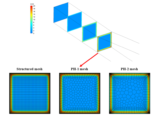
Figure 12.156: Streamlines of crossflow pattern at the start of the diffuser for three different meshes.
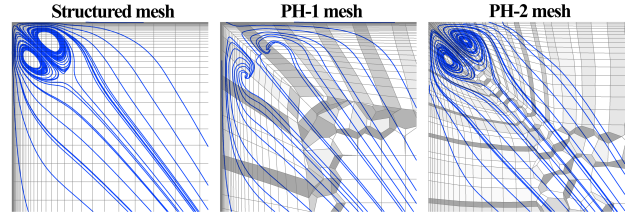
Figure 12.157: Distribution of the skin friction along the diffuser at midsection (left) and near the corner (right) for SST-CFC for the DLR diffuser for two unstructured and one structured mesh [41].
![Distribution of the skin friction along the diffuser at midsection (left) and near the corner (right) for SST-CFC for the DLR diffuser for two unstructured and one structured mesh [].](graphics/image192.5.png)
Figure 12.158: Distribution of the pressure coefficient along the diffuser at midsection for SST-CFC for the DLR diffuser for two unstructured and one structured mesh [41].
![Distribution of the pressure coefficient along the diffuser at midsection for SST-CFC for the DLR diffuser for two unstructured and one structured mesh [].](graphics/image194.png)