


The following topics are discussed:
- 12.3.2.1. The 'Separation' Parameter CSEP
- 12.3.2.2. 3.2 The 'Near Wall' Parameter CNW
- 12.3.2.3. The 'Mixing' Parameter CMIX
- 12.3.2.4. The 'Jet' Parameter CJET
- 12.3.2.5. The 'Corner' Parameter CCORNER
- 12.3.2.6. The 'Curvature' Parameter CCURV
- 12.3.2.7. The Blending Function
- 12.3.2.8. Other Special Coefficients
The ability to predict separation depends mostly on the level of the eddy-viscosity in
the boundary layer. A suitable approach for tuning the model to adverse pressure
gradients and separation is to allow a re-calibration of the basic model constants,
while at the same time maintaining the calibration for the slope of the logarithmic
layer and the proper near wall viscous damping required for achieving the correct shift
in the log-layer (and thereby the correct wall shear stress). This is achieved by using
the free parameter  .
.
Figure 12.172: Change of the eddy-viscosity ration (EVR) under changes of  for a flat plate. Top:
 =1.0 (all else default). Bottom
  =1.75 (all else default) shows the effect of
  on a flat plate boundary layer computation for the ratio
  . Increasing
  from
from  =1.00 to
  =1.75 leads to a significant reduction in the ER levels. (Note that the effect
is even more pronounced for flows with adverse pressure gradients and separation).
=1.75 leads to a significant reduction in the ER levels. (Note that the effect
is even more pronounced for flows with adverse pressure gradients and separation).
Figure 12.172: Change of the eddy-viscosity ration (EVR) under changes of for a flat plate. Top:=1.0 (all else default). Bottom =1.75 (all else default)
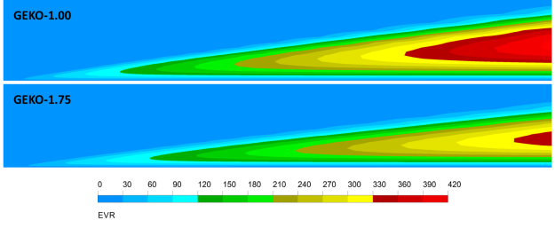
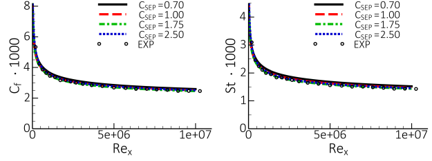
Figure 12.173: Flat plate boundary layer under variation of  (
( =0.5). Left: Wall-shear stress coefficient,
  , Right: Wall heat transfer coefficient, St shows that even large changes in
  do not have any effect on the wall shear stress (
 )
and heat transfer coefficients (St). This is the basic design criterion for the GEKO model. It
ensures that the user can adjust coefficients like
)
and heat transfer coefficients (St). This is the basic design criterion for the GEKO model. It
ensures that the user can adjust coefficients like  freely (within range).
Figure 12.173: Flat plate boundary layer under variation of (=0.5). Left: Wall-shear stress coefficient, , Right: Wall heat transfer coefficient, St
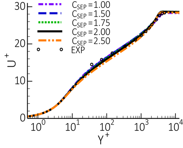
The independence of the mean flow velocity is also illustrated by the
logarithmic velocity profiles shown in Figure 12.174: Velocity profiles in logarithmic plot under variation of  for flat plate. Again, the logarithmic velocity profile is maintained
over a wide range of
for flat plate. Again, the logarithmic velocity profile is maintained
over a wide range of  coefficients.
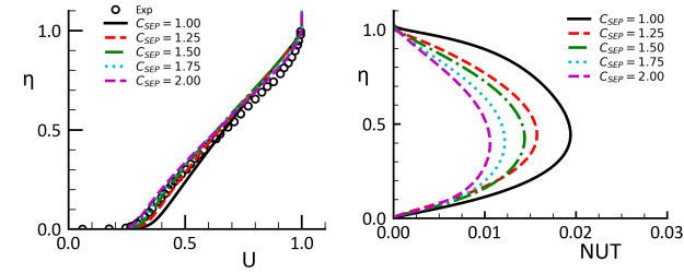
The effect of  on an equilibrium adverse pressure-gradient boundary layer flows is
demonstrated for the experiment of Skare and Krogstad (
on an equilibrium adverse pressure-gradient boundary layer flows is
demonstrated for the experiment of Skare and Krogstad ( ) [21]. The
simulations are based on the equilibrium boundary layer equations as given by Wilcox
[31]. The non-dimensional pressure gradient
) [21]. The
simulations are based on the equilibrium boundary layer equations as given by Wilcox
[31]. The non-dimensional pressure gradient  drives the flow close to separation,
a regime, which is very sensitive to turbulence modeling. The left part of Figure 12.175: Impact of variation in
drives the flow close to separation,
a regime, which is very sensitive to turbulence modeling. The left part of Figure 12.175: Impact of variation in  on boundary layer with adverse pressure gradient. Left: Velocity profile. Right Eddy-viscosity profiles
shows the influence of
on boundary layer with adverse pressure gradient. Left: Velocity profile. Right Eddy-viscosity profiles
shows the influence of  on the velocity profiles whereas the right part shows the
impact on the non-dimensional eddy-viscosity,
on the velocity profiles whereas the right part shows the
impact on the non-dimensional eddy-viscosity,  (
( is the
velocity at the edge of the boundary layer and
is the
velocity at the edge of the boundary layer and  is the displacement thickness). The
velocity profile exhibits moderately but visibly more decelerated with increasing
is the displacement thickness). The
velocity profile exhibits moderately but visibly more decelerated with increasing
 . The eddy-viscosity, however, is drastically reduced by more than a factor of
two by the variation of
. The eddy-viscosity, however, is drastically reduced by more than a factor of
two by the variation of  between 1-2. The most accurate solution is the one with
 =1.75. This reduction in eddy-viscosity is desirable for adverse pressure-gradient
boundary layers, as low values increase the sensitivity of the model to adverse
pressure gradients and separation. Note that the coefficients
=1.75. This reduction in eddy-viscosity is desirable for adverse pressure-gradient
boundary layers, as low values increase the sensitivity of the model to adverse
pressure gradients and separation. Note that the coefficients  ,
,  have little
effect on the boundary layer flows, due to the blending function being mostly equal to
one inside the boundary layer. The parameter
have little
effect on the boundary layer flows, due to the blending function being mostly equal to
one inside the boundary layer. The parameter  was set to its default value
  =0.5
(as will be detailed later). However, variations of
=0.5
(as will be detailed later). However, variations of  would have little effect on
the current flow.
would have little effect on
the current flow.
Figure 12.175: Impact of variation in on boundary layer with adverse pressure gradient. Left: Velocity profile. Right Eddy-viscosity profiles
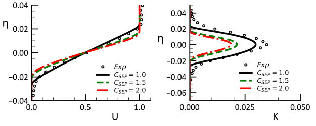
The effect of variation in  is shown in Figure 12.176: Impact of variation in
 ![Impact of variation in on CS0 diffuser flow []. Left wall shear stress coefficient, . Right: Wall pressure coefficient](graphics/eq5e08a44b-8708-4780-aba7-ebb9577ab239.svg) on CS0 diffuser flow [10]. Left wall shear stress coefficient,
on CS0 diffuser flow [10]. Left wall shear stress coefficient, ![Impact of variation in on CS0 diffuser flow []. Left wall shear stress coefficient, . Right: Wall pressure coefficient](graphics/eq3702f87a-6bc6-4c42-9970-bcd5ecf1bd54.svg) . Right: Wall pressure coefficient
. Right: Wall pressure coefficient ![Impact of variation in on CS0 diffuser flow []. Left wall shear stress coefficient, . Right: Wall pressure coefficient](graphics/eqc227a095-c282-4308-bd8e-bd5186e65b60.svg) for the axi-symmetric diffuser
flow of Driver et al [10] (
for the axi-symmetric diffuser
flow of Driver et al [10] ( =0.5,
=0.5,  =CMixCor,
  =0.9). As expected from the
results for the equilibrium boundary layer, with increasing
=0.9). As expected from the
results for the equilibrium boundary layer, with increasing  , the model becomes
more sensitive to the adverse pressure gradient in the diffuser and improves its
separation predict up to a value of
, the model becomes
more sensitive to the adverse pressure gradient in the diffuser and improves its
separation predict up to a value of  ~1.75-2.00. Higher values of
  lead to
over-separation. Note that an optimal calibration of a turbulence model for the CS0
diffuser, does not necessarily guarantee an optimal solution for other similar
flows. As will be shown below, for 2D airfoils more 'aggressive' settings are
required to match the exp. data. It is therefore desirable that the GEKO model can
be pushed to over-separation for the CS0 case.
lead to
over-separation. Note that an optimal calibration of a turbulence model for the CS0
diffuser, does not necessarily guarantee an optimal solution for other similar
flows. As will be shown below, for 2D airfoils more 'aggressive' settings are
required to match the exp. data. It is therefore desirable that the GEKO model can
be pushed to over-separation for the CS0 case.
Figure 12.176: Impact of variation in on CS0 diffuser flow [10]. Left wall shear stress coefficient, . Right: Wall pressure coefficient
![Impact of variation in on CS0 diffuser flow []. Left wall shear stress coefficient, . Right: Wall pressure coefficient](graphics/image039.5.png)
![Impact of variation in on velocity profiles for CS0 diffuser flow []](graphics/eqc2c32336-a1ea-454c-8c3e-b3b75a2df3b1.svg)
![Impact of variation in on velocity profiles for CS0 diffuser flow []](graphics/image041.png)
A more realistic application for tuning the  coefficient is the simulation of 2D
airfoil profiles under variation of the angle of attack,
coefficient is the simulation of 2D
airfoil profiles under variation of the angle of attack,  . Figure 12.178: Prediction of lift and pressure coefficients with GEKO model for DU-96-W-180 (Left) and DU-97-W-300 (Right) airfoil at
 ![Prediction of lift and pressure coefficients with GEKO model for DU-96-W-180 (Left) and DU-97-W-300 (Right) airfoil at []](graphics/eq956ec826-aa31-4057-9de7-20c4aae85edf.svg) [28] to Figure 12.182: Prediction of lift coefficient in wide range of angle of attacks (Left) and pressure coefficient for
[28] to Figure 12.182: Prediction of lift coefficient in wide range of angle of attacks (Left) and pressure coefficient for ![Prediction of lift coefficient in wide range of angle of attacks (Left) and pressure coefficient for (Right) with GEKO model for S814 airfoil at []](graphics/eq6b6b51a0-1692-4bed-bd5a-f7a36d3aff0e.svg) (Right) with GEKO model for S814 airfoil at
(Right) with GEKO model for S814 airfoil at ![Prediction of lift coefficient in wide range of angle of attacks (Left) and pressure coefficient for (Right) with GEKO model for S814 airfoil at []](graphics/eq11c8e6ae-efbf-4f4f-bd15-3f3cf28752c4.svg) [26]
compare lift curves for numerous airfoils computed with the GEKO model. In these
comparisons, it should be kept in mind that 2D simulations are not entirely correct
in the stall and post-stall region (around and past maximum lift,
[26]
compare lift curves for numerous airfoils computed with the GEKO model. In these
comparisons, it should be kept in mind that 2D simulations are not entirely correct
in the stall and post-stall region (around and past maximum lift,  ), due to the
formation of 3D structures in the experiments. Despite of this, it is possible to
adjust the GEKO model for the prediction of such flows for angles of attack in 2D
simulations. Increasing
), due to the
formation of 3D structures in the experiments. Despite of this, it is possible to
adjust the GEKO model for the prediction of such flows for angles of attack in 2D
simulations. Increasing  predicts earlier separation onset, which improves
agreement of the predicted pressure coefficient and results in an improved agreement
of the lift coefficient with the experimental data[5] near stall.
The optimal value for
predicts earlier separation onset, which improves
agreement of the predicted pressure coefficient and results in an improved agreement
of the lift coefficient with the experimental data[5] near stall.
The optimal value for  for such flows is therefore somewhere between
 =2.00-2.50.
The current test cases demonstrate the advantage of the GEKO model over e.g. the SST
model. The SST model is tuned to match adverse pressure gradients flows and flows with
separation well on average. However, for the 2D airfoils the SST model is clearly too
conservative resulting in overly optimistic CLmax levels. This would be hard to correct
within the SST model and in any case would require expert knowledge in turbulence
modeling. Within the GEKO model, separation prediction can easily be adjusted by
changing  even by a non-expert.
Figure 12.178: Prediction of lift and pressure coefficients with GEKO model for DU-96-W-180 (Left) and DU-97-W-300 (Right) airfoil at [28]
![Prediction of lift and pressure coefficients with GEKO model for DU-96-W-180 (Left) and DU-97-W-300 (Right) airfoil at []](graphics/image042.5.png)
Figure 12.179: Prediction of lift coefficient in wide range of angle of attacks (Left) and pressure coefficient for ![Prediction of lift coefficient in wide range of angle of attacks (Left) and pressure coefficient for (Right) with GEKO model for S805 airfoil at []](graphics/eq9bb30bcc-265a-40f3-832a-833c3d72c0e5.svg) (Right) with GEKO model for S805 airfoil at
(Right) with GEKO model for S805 airfoil at ![Prediction of lift coefficient in wide range of angle of attacks (Left) and pressure coefficient for (Right) with GEKO model for S805 airfoil at []](graphics/eqdd3addab-1164-42c6-98e7-05f6e84f236d.svg) [23]
[23]
![Prediction of lift coefficient in wide range of angle of attacks (Left) and pressure coefficient for (Right) with GEKO model for S805 airfoil at []](graphics/image044.png)
Figure 12.180: Prediction of lift coefficient wide range of angle of attacks (Left) and pressure coefficient for ![Prediction of lift coefficient wide range of angle of attacks (Left) and pressure coefficient for (Right) with GEKO model for S825 airfoil at []](graphics/eq848cce1a-2dfd-4ab2-bbe4-d87d5e67cdb9.svg) (Right) with GEKO model for S825 airfoil at
(Right) with GEKO model for S825 airfoil at ![Prediction of lift coefficient wide range of angle of attacks (Left) and pressure coefficient for (Right) with GEKO model for S825 airfoil at []](graphics/eq0d0413a6-1c7d-4a04-a3a2-2464e231fe04.svg) [24]
[24]
![Prediction of lift coefficient wide range of angle of attacks (Left) and pressure coefficient for (Right) with GEKO model for S825 airfoil at []](graphics/image045.png)
Figure 12.181: Prediction of lift coefficient in wide range of angle of attacks (Left) and pressure coefficient for ![Prediction of lift coefficient in wide range of angle of attacks (Left) and pressure coefficient for (Right) with GEKO model for S809 airfoil at []](graphics/eq1aa71dc7-0e1d-44ca-89ed-b8640311b287.svg) (Right) with GEKO model for S809 airfoil at
(Right) with GEKO model for S809 airfoil at ![Prediction of lift coefficient in wide range of angle of attacks (Left) and pressure coefficient for (Right) with GEKO model for S809 airfoil at []](graphics/eqee27d623-4bc8-4184-ae17-94005179fa80.svg) [25]
[25]
![Prediction of lift coefficient in wide range of angle of attacks (Left) and pressure coefficient for (Right) with GEKO model for S809 airfoil at []](graphics/image046.png)
Figure 12.182: Prediction of lift coefficient in wide range of angle of attacks (Left) and pressure coefficient for (Right) with GEKO model for S814 airfoil at [26]
![Prediction of lift coefficient in wide range of angle of attacks (Left) and pressure coefficient for (Right) with GEKO model for S814 airfoil at []](graphics/image047.png)
It is important to understand that changes of  affect not only boundary layers, but
the entire flow field. Increasing
affect not only boundary layers, but
the entire flow field. Increasing  reduces the eddy-viscosity in all parts of the
domain, including for free shear flows (e.g. mixing layers etc.). Frequently, the
adjustment of boundary layer separation is the main optimization requirement and it is
desirable to maintain the performance and calibration for free shear flows (e.g.
spreading rates for mixing layers and jets etc.). In order to avoid any negative impact
of
reduces the eddy-viscosity in all parts of the
domain, including for free shear flows (e.g. mixing layers etc.). Frequently, the
adjustment of boundary layer separation is the main optimization requirement and it is
desirable to maintain the performance and calibration for free shear flows (e.g.
spreading rates for mixing layers and jets etc.). In order to avoid any negative impact
of  on free shear flows, the reduction in eddy-viscosity is corrected by modifying
 accordingly. This is achieved through the correlation
  given in Equation
(2.11). This correlation increases
given in Equation
(2.11). This correlation increases  with increasing
  to maintain the spreading
rates for mixing layers. As the correlation
to maintain the spreading
rates for mixing layers. As the correlation  =CMixCor is default, users do not
have to adjust
=CMixCor is default, users do not
have to adjust  when changing
  . This effect will be demonstrated in the
Section 3.3 dealing with the impact of
. This effect will be demonstrated in the
Section 3.3 dealing with the impact of  .
.
The Bachalo-Johnson NASA Bump flow experiment [2], as depicted in Figure 12.183: Schematic of transonic axi-symmetric bump flow, features a
subsonic inflow with Ma=0.875. The flow is then accelerated to supersonic speed over
the bump and then reverts to subsonic speed through a shock wave. The shock causes the
boundary layer behind the shock to separate, which in turn interacts with the shock by
pushing it forward. The ability to predict the shock location is therefore directly
linked to a model's ability to predict boundary layer separation. As expected, again,
the models group as GEKO-1.75/SST and GEKO-1.00/RKE as seen from Figure 12.184: Pressure coefficient,![Pressure coefficient,, along wall of bump. Comparison of different GEKO settings with RKE and SST model and experimental data [].](graphics/eq2f1a15b9-8728-4cc3-b8a0-67d30337872c.svg) , along wall of bump. Comparison of different GEKO settings with RKE and SST model and experimental data [2].. Both, the
GEKO-1.75 and the SST model can predict the shock location and the post-shock
separation zone properly. The GEKO-1.00/RKE models fail due to their lack of separation
sensitivity.
, along wall of bump. Comparison of different GEKO settings with RKE and SST model and experimental data [2].. Both, the
GEKO-1.75 and the SST model can predict the shock location and the post-shock
separation zone properly. The GEKO-1.00/RKE models fail due to their lack of separation
sensitivity.
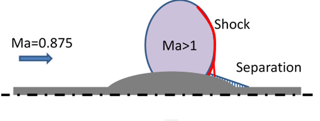
Figure 12.184: Pressure coefficient,, along wall of bump. Comparison of different GEKO settings with RKE and SST model and experimental data [2].
![Pressure coefficient,, along wall of bump. Comparison of different GEKO settings with RKE and SST model and experimental data [].](graphics/image049.png)
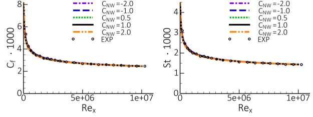
The coefficient  is introduced to allow a modification of the model characteristics
in the near wall region under non-equilibrium conditions. It has a strong effect on
heat transfer predictions in reattachment and stagnation regions.
is introduced to allow a modification of the model characteristics
in the near wall region under non-equilibrium conditions. It has a strong effect on
heat transfer predictions in reattachment and stagnation regions.
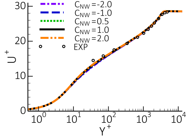
The first task is to show that variations in  (like
(like  ) do not affect flat plate
boundary layer behavior. This can be seen from Figure 12.185: Flat plate boundary layer under variation of
) do not affect flat plate
boundary layer behavior. This can be seen from Figure 12.185: Flat plate boundary layer under variation of  (
( =1.75). Left: Wall-shear stress coefficient,
  , Right: Wall heat transfer coefficient, St. where both, the wall shear
stress coefficient,
, Right: Wall heat transfer coefficient, St. where both, the wall shear
stress coefficient, , and the wall heat transfer coefficient St are unaffected by
variations in
, and the wall heat transfer coefficient St are unaffected by
variations in  . In addition, the velocity profile in log-scale is maintained as
shown in Figure 12.186: Velocity profiles in logarithmic coordinates - variation of
. In addition, the velocity profile in log-scale is maintained as
shown in Figure 12.186: Velocity profiles in logarithmic coordinates - variation of  (
( =1.75). Many more variations of parameters
  and
and  have been tested
and the agreement is like that shown in Figure 12.186: Velocity profiles in logarithmic coordinates - variation of (=1.75).
have been tested
and the agreement is like that shown in Figure 12.186: Velocity profiles in logarithmic coordinates - variation of (=1.75).
Figure 12.185: Flat plate boundary layer under variation of (=1.75). Left: Wall-shear stress coefficient, , Right: Wall heat transfer coefficient, St.
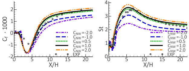
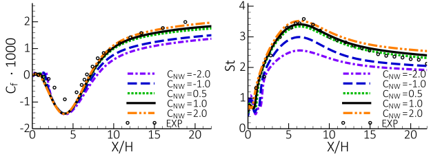
The effect of changing  for the axisymmetric diffuser test case CS0 [10] is shown in Figure 12.187: Impact of variation in
 ![Impact of variation in on CS0 diffuser flow []. Left: Wall shear-stress coefficient, . Right: Wall pressure coefficient (=1.0, =0.0, =0.9)](graphics/eq988eac40-5dd7-4728-a5d8-339fe599ddce.svg) on CS0 diffuser flow [10]. Left: Wall shear-stress coefficient,
on CS0 diffuser flow [10]. Left: Wall shear-stress coefficient, ![Impact of variation in on CS0 diffuser flow []. Left: Wall shear-stress coefficient, . Right: Wall pressure coefficient (=1.0, =0.0, =0.9)](graphics/eq62e9642f-accb-4756-9cee-03a6541c2d02.svg) . Right: Wall pressure coefficient
. Right: Wall pressure coefficient ![Impact of variation in on CS0 diffuser flow []. Left: Wall shear-stress coefficient, . Right: Wall pressure coefficient (=1.0, =0.0, =0.9)](graphics/eqccb1b28c-d754-4821-bb6e-24b1e6b9ab49.svg) (
(![Impact of variation in on CS0 diffuser flow []. Left: Wall shear-stress coefficient, . Right: Wall pressure coefficient (=1.0, =0.0, =0.9)](graphics/eq92f0e5e1-ae4f-4c4f-87e1-53bb6d5d0f0e.svg) =1.0,
=1.0, ![Impact of variation in on CS0 diffuser flow []. Left: Wall shear-stress coefficient, . Right: Wall pressure coefficient (=1.0, =0.0, =0.9)](graphics/eq31694005-f041-4d11-b508-ddf4571b3bd3.svg) =0.0,
=0.0, ![Impact of variation in on CS0 diffuser flow []. Left: Wall shear-stress coefficient, . Right: Wall pressure coefficient (=1.0, =0.0, =0.9)](graphics/eq318b308b-0ec5-4ddf-a25f-cca55fd05f8d.svg) =0.9). The coefficient
=0.9). The coefficient  is designed to have an influence mostly near the wall. Therefore, the wall
shear-stress distribution shows a much larger sensitivity to this variation (Figure 12.187: Impact of variation in on CS0 diffuser flow [10]. Left: Wall shear-stress coefficient, . Right: Wall pressure coefficient (=1.0, =0.0, =0.9) Left) than the Cp-distribution (Figure 12.187: Impact of variation in on CS0 diffuser flow [10]. Left: Wall shear-stress coefficient, . Right: Wall pressure coefficient (=1.0, =0.0, =0.9)
Right). The velocity profiles shown in Figure 12.188: Impact of variation in
is designed to have an influence mostly near the wall. Therefore, the wall
shear-stress distribution shows a much larger sensitivity to this variation (Figure 12.187: Impact of variation in on CS0 diffuser flow [10]. Left: Wall shear-stress coefficient, . Right: Wall pressure coefficient (=1.0, =0.0, =0.9) Left) than the Cp-distribution (Figure 12.187: Impact of variation in on CS0 diffuser flow [10]. Left: Wall shear-stress coefficient, . Right: Wall pressure coefficient (=1.0, =0.0, =0.9)
Right). The velocity profiles shown in Figure 12.188: Impact of variation in ![Impact of variation in on velocity profiles for CS0 diffuser flow []](graphics/eq7e3d044d-ce9f-456c-8e2d-79459ae7030b.svg) on velocity profiles for CS0 diffuser flow [10] illustrate the effect
more clearly. Contrary to changes of
on velocity profiles for CS0 diffuser flow [10] illustrate the effect
more clearly. Contrary to changes of  , where the entire boundary layer is affected, variations in
  change only the inner part of the velocity profiles.
Figure 12.187: Impact of variation in on CS0 diffuser flow [10]. Left: Wall shear-stress coefficient, . Right: Wall pressure coefficient (=1.0, =0.0, =0.9)
![Impact of variation in on CS0 diffuser flow []. Left: Wall shear-stress coefficient, . Right: Wall pressure coefficient (=1.0, =0.0, =0.9)](graphics/image053.5.png)
![Impact of variation in on velocity profiles for CS0 diffuser flow []](graphics/image055.png)
For non-equilibrium flows, the wall shear stress and more importantly, the heat
transfer to a wall, depend mostly on the model details close to the wall. The
coefficient  can be tuned to allow fine-tuning for such flows. An example is
backward-facing step with Cf and heat transfer measurements, St, downstream of
the step [31]. The effect is shown in Figure 12.189: Backward-facing step with heat transfer under variation of
can be tuned to allow fine-tuning for such flows. An example is
backward-facing step with Cf and heat transfer measurements, St, downstream of
the step [31]. The effect is shown in Figure 12.189: Backward-facing step with heat transfer under variation of  (Top:
(Top: =1.00, Bottom:
  =1.75, Both:
  =0.9,
=0.9,  =
= ). Left: Wall shear stress coefficient,
  , Right: Heat transfer Stanton number. It is computed with both,
 =1.0 and
  =1.75,
  =CMixCor ,
  =0.9 and a variation in
  . The
heat transfer is strongly affected (and can therefore be optimized) by changes
in
. The
heat transfer is strongly affected (and can therefore be optimized) by changes
in  . In the current application, the optimal value is
  =0.5 for both
values of
=0.5 for both
values of  .
.  =0.5 is also the default setting. It is important to note
that
=0.5 is also the default setting. It is important to note
that  is a minor parameter and will likely not have to be tuned for most
flows. Wider validation studies indicate that the default value is suitable for most
applications.
is a minor parameter and will likely not have to be tuned for most
flows. Wider validation studies indicate that the default value is suitable for most
applications.

Figure 12.189: Backward-facing step with heat transfer under variation of (Top:=1.00, Bottom: =1.75, Both: =0.9, =). Left: Wall shear stress coefficient, , Right: Heat transfer Stanton number

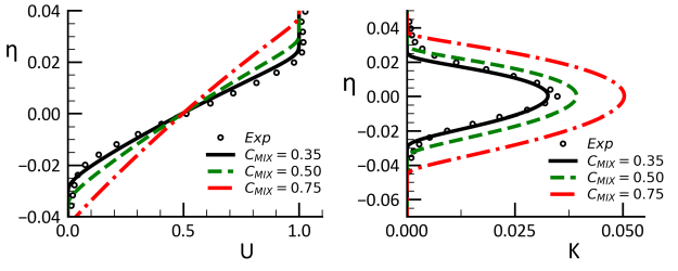
The parameter  affects only free shear flows. It has no impact on boundary layers
due to the blending function FBlend. Increasing
affects only free shear flows. It has no impact on boundary layers
due to the blending function FBlend. Increasing  leads to larger eddy-viscosity
(higher turbulence levels) in free shear flows. This is illustrated in Figure 12.190: Impact of variation in
leads to larger eddy-viscosity
(higher turbulence levels) in free shear flows. This is illustrated in Figure 12.190: Impact of variation in  on mixing layer when using the
  =2(
=2( =0.9,
=0.9,  =0.5). Left: Velocity profile. Right: Turbulence kinetic energy profiles which
shows results for a mixing layer simulation compared with experimental data [3]. As
expected, increasing
=0.5). Left: Velocity profile. Right: Turbulence kinetic energy profiles which
shows results for a mixing layer simulation compared with experimental data [3]. As
expected, increasing  leads to larger spreading rates of the velocity profile,
associated with higher levels of turbulence kinetic energy. In most applications, it is
desirable to calibrate the coefficient such that a good agreement with mixing layer
flows is achieved (in the current example with
leads to larger spreading rates of the velocity profile,
associated with higher levels of turbulence kinetic energy. In most applications, it is
desirable to calibrate the coefficient such that a good agreement with mixing layer
flows is achieved (in the current example with  =2 this means
  =0.35). However,
there can be cases, where stronger mixing is desired and where the calibration for a
classical mixing layer is not sufficient. Examples are flows with strong mixing
characteristics, like flows past bluff bodies etc. It should be emphasized that the
physical reason for increased mixing in such cases is often a result of flow
unsteadiness (e.g. vortex shedding) augmenting the conventional turbulence mixing.
In such cases it will not be possible to obtain a perfect agreement against data, as
such unsteady effects are typically stronger than that which a turbulence model can
provide. Still, increasing
=0.35). However,
there can be cases, where stronger mixing is desired and where the calibration for a
classical mixing layer is not sufficient. Examples are flows with strong mixing
characteristics, like flows past bluff bodies etc. It should be emphasized that the
physical reason for increased mixing in such cases is often a result of flow
unsteadiness (e.g. vortex shedding) augmenting the conventional turbulence mixing.
In such cases it will not be possible to obtain a perfect agreement against data, as
such unsteady effects are typically stronger than that which a turbulence model can
provide. Still, increasing  can at least compensate for some of the missing
effects, in case that unsteady (scale resolving) simulations are not feasible.
can at least compensate for some of the missing
effects, in case that unsteady (scale resolving) simulations are not feasible.
Figure 12.190: Impact of variation in on mixing layer when using the =2(=0.9, =0.5). Left: Velocity profile. Right: Turbulence kinetic energy profiles
As already mentioned in the section on  (section 3.1), there is a subtle
interaction of
(section 3.1), there is a subtle
interaction of  and
and  which users have to understand. Variations in
 also affect free shear flows and increases in
  result in lower
spreading rates. This can be seen in Figure 12.191: Impact of variation in
result in lower
spreading rates. This can be seen in Figure 12.191: Impact of variation in  on mixing layer (
 =0,
=0,  =0.9,
=0.9,  =0.5). Left: Velocity profile. Right: Turbulence kinetic energy profiles which shows the results of a
 variation for the mixing layer [3] (
 = 0,
= 0,  = 0.9,
  = 0.5).
Here the solution with
= 0.5).
Here the solution with  = 1 is closest to the data whereas the solution
with
= 1 is closest to the data whereas the solution
with  =2 predicts far too low spreading rates and turbulence levels. The
effect on the eddy-viscosity is even stronger than for the boundary layer
resulting in a reduction of more than a factor 3 with increasing
=2 predicts far too low spreading rates and turbulence levels. The
effect on the eddy-viscosity is even stronger than for the boundary layer
resulting in a reduction of more than a factor 3 with increasing  (not
shown).
(not
shown).
Figure 12.191: Impact of variation in on mixing layer (=0, =0.9, =0.5). Left: Velocity profile. Right: Turbulence kinetic energy profiles
In order to compensate the effect of  on free shear flows, the coefficient
  has
to be increased with increasing
has
to be increased with increasing  . This is achieved by the correlation CMixCor given
in Equation (2.11) which is the model default. The correlation is provided so that
users know which value is optimal for a given
. This is achieved by the correlation CMixCor given
in Equation (2.11) which is the model default. The correlation is provided so that
users know which value is optimal for a given  setting. Increasing
  above this
value will lead to higher and decreasing it to lower turbulence levels and spreading
rates for free shear flows.
above this
value will lead to higher and decreasing it to lower turbulence levels and spreading
rates for free shear flows.
The results for mixing layer simulations with  = CMixCor are shown in Figure 12.192: Impact of variation in
  on mixing layer when using the
  =
= correlation (
 =0.9,
=0.9,  =0.5). Left: Velocity profile. Right: Turbulence kinetic energy profiles. For
all selected values of
=0.5). Left: Velocity profile. Right: Turbulence kinetic energy profiles. For
all selected values of  , the mixing layer is maintained, and correct spreading
rates are achieved.
, the mixing layer is maintained, and correct spreading
rates are achieved.
Figure 12.192: Impact of variation in on mixing layer when using the = correlation (=0.9, =0.5). Left: Velocity profile. Right: Turbulence kinetic energy profiles
The impact of the  parameter is subtle and in most applications it can be
maintained at its default value. It is important in cases where jet flows need to be
computed with high accuracy. Remember that conventional models like
parameter is subtle and in most applications it can be
maintained at its default value. It is important in cases where jet flows need to be
computed with high accuracy. Remember that conventional models like  or SST will
over-predict spreading rates of round jets substantially while giving reasonable
results for plane jets. For this so-called round-jet plane-jet 'anomaly' see e.g.
[19,33].
or SST will
over-predict spreading rates of round jets substantially while giving reasonable
results for plane jets. For this so-called round-jet plane-jet 'anomaly' see e.g.
[19,33].
The GEKO model is designed to provide parameter settings which allow an accurate
representation of jet flow. This is achieved through the parameter  . The way this
is achieved is by reducing the influence of
. The way this
is achieved is by reducing the influence of  (which increases mixing layer
spreading rates) on jet flows (especially round jets). It should also be noted that the
coefficient
(which increases mixing layer
spreading rates) on jet flows (especially round jets). It should also be noted that the
coefficient  is a sub-function of the coefficient
  . In case
  =0, the
coefficient
=0, the
coefficient  has no impact.
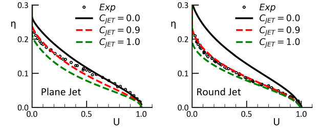
Simulations are again based on self-similar jet-flow equations as given by
Wilcox [33]. The two test cases are Wygnanski and Fielder [36] for the plane jet and Bradbury
[4] for the round jet. Figure 12.193: Effect of  for plane (left) and round (right) jet flow (
 =2.0,
=2.0,  =0.35,
  =0.5) shows simulations with
  =2,
=2,  =0.35 (Correlation) and
  =0.5 (default). It is clearly seen that the model overpredicts the spreading
rates especially for the round jet with
=0.5 (default). It is clearly seen that the model overpredicts the spreading
rates especially for the round jet with  =0. The effect of
  is to reduce the spreading rate of both jet flows, with
  =0.9 being close to both experimental data-sets. With
  =2 and
  =0.9, the model avoids the round jet/plane jet anomaly and predicts lower
spreading rates for the round than for the plane jet. Note again, that the changes of
=0.9, the model avoids the round jet/plane jet anomaly and predicts lower
spreading rates for the round than for the plane jet. Note again, that the changes of
 discussed here do not affect the mixing layer.
In contrast, Figure 12.194: Comparison of GEKO-1 and GEKO-2 model (with variation of  =0.9) shows a comparison between GEKO-1 (
 =1.0) and GEKO-2
(
=1.0) and GEKO-2
( =1.0) with
  =0.9. As GEKO-1 is a close cousin of the standard
  model it
behaves just like that model. It gives a correct spreading rate for the plane jet but
over-predicts the round jet. Note again, that changes to
model it
behaves just like that model. It gives a correct spreading rate for the plane jet but
over-predicts the round jet. Note again, that changes to  in GEKO-1 would have no
effect, as for that model
in GEKO-1 would have no
effect, as for that model  =0 (so that the sub-model
  is de-activated).
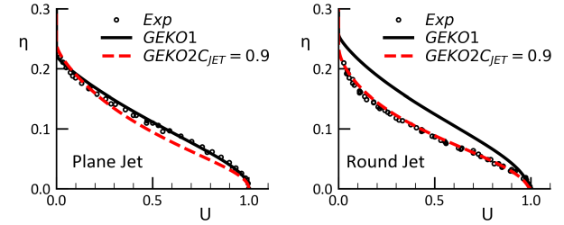
In summary, in order to achieve optimal performance for round jets, one needs to set
 to values
  ~1.75-2.00 and
  =0.9 (default). With reduction in
  and the
corresponding reduction in
and the
corresponding reduction in  , the effect of
  vanishes.
There is another parameter CJET_AUX which also has an influence on the jet flow. It
defines the limit between mixing layers and jet flows. The larger the value, the
sharper the 'demarcation' and stronger the effect of  . The default value is
CJET_AUX =2.0. It is suitable for jet flow simulations to set the value to
CJET_AUX =4.0. This is not done by default, as it can lead to oscillations on poor
meshes.
. The default value is
CJET_AUX =2.0. It is suitable for jet flow simulations to set the value to
CJET_AUX =4.0. This is not done by default, as it can lead to oscillations on poor
meshes.
Users who do not have a need for accurate predictions of jets can use the default
settings for  .
.
It is well known that for rectangular turbulent channel flows, secondary flows develop in the plane normal to the mean flow. Such secondary flow is not present in laminar flows and can also not be represented at all by eddy-viscosity models. The situation is depicted in Figure 12.195: Comparison of streamline velocity contours and secondary motion predicted by linear (Left) and non-linear (Center) GEKO-1.00 model with the DNS (Right) data in the fully developed square duct flow [19] for a square channel. The main flow direction is normal to the plotting plane. The velocity contour colors on the left picture show the main flow as computed by a linear eddy-viscosity model. There are no streamlines when projected into this plane.
The practical effect of this effect is that the secondary flow transports flow (and thereby momentum) into the corner. If the corner flow experiences an adverse pressure gradient, this additional momentum can help the flow to avoid/delay separation. When computing such flows with an eddy-viscosity model, such separations can occur earlier than in the experiments, which in turn can have a substantial effect on the overall performance. The right picture shows the results from a Direct Numerical Simulation (DNS, e.g. [19]) of this flow. There are clearly recognizable secondary streamlines pushing flow into the corners. The center picture shows the GEKO model in combination with an existing non-linear algebraic stress-strain model (Wallin-Johansson Explicit Reynolds Stress Models WJ-EARSM), which can mimic the effect. The WJ-EARSM is fairly complex and the GEKO model was used as a reference point for calibration of the much simpler quadratic stress-strain relationship which can also account for this effect (Equation (2.7)). This term has a free parameter, CCORNER, which can be tuned by the users.
Figure 12.195: Comparison of streamline velocity contours and secondary motion predicted by linear (Left) and non-linear (Center) GEKO-1.00 model with the DNS (Right) data in the fully developed square duct flow [19]
![Comparison of streamline velocity contours and secondary motion predicted by linear (Left) and non-linear (Center) GEKO-1.00 model with the DNS (Right) data in the fully developed square duct flow []](graphics/image070.5.png)
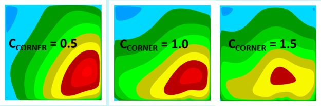
Figure 12.196: Comparison of turbulence models for flow in square channel. Left: GEKO with WJ-EARSM. Middle, GEKO with CCORER=0.9. Right GEKO linear (CCORNER=0.0). shows a comparison for the rectangular channel for GEKO-175 ( =1.75 all
else default). The left picture shows the combination of GEKO with the WJ-EARSM, the
middle picture the combination with the quadratic term and CCORNER=0.9 and the left
for CCORNER=0.0. The simple quadratic model gives a good approximation of the flow,
similar to the WJ-EARSM.
=1.75 all
else default). The left picture shows the combination of GEKO with the WJ-EARSM, the
middle picture the combination with the quadratic term and CCORNER=0.9 and the left
for CCORNER=0.0. The simple quadratic model gives a good approximation of the flow,
similar to the WJ-EARSM.
Figure 12.196: Comparison of turbulence models for flow in square channel. Left: GEKO with WJ-EARSM. Middle, GEKO with CCORER=0.9. Right GEKO linear (CCORNER=0.0).
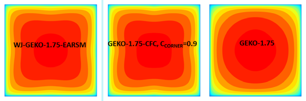
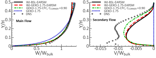
Figure 12.197: Velocity profiles plotted along diagonal of channel for different turbulence models against DNS data. Right: Main flow, Left Secondary Flow shows a comparison of velocity profiles for different turbulence models for
the square channel. The right part of the picture shows the secondary flow into the
corner along a diagonal of the channel cross-section. Most obviously, the linear model
(GEKO-1.75) gives zero velocity along the diagonal. The other models provide fairly
similar strength and distributions of the same order as the reference DNS data, but
clearly also not in perfect agreement, especially very close to the wall. Note that
further increases in  for this flow would break the symmetry of the crossflow
pattern. The left part of the figure shows the mean flow profile also along the
diagonal. The most important effect is the higher velocity close to the wall
('fuller profile') which allows the flow to overcome a stronger pressure gradient
before separating.
for this flow would break the symmetry of the crossflow
pattern. The left part of the figure shows the mean flow profile also along the
diagonal. The most important effect is the higher velocity close to the wall
('fuller profile') which allows the flow to overcome a stronger pressure gradient
before separating.
Figure 12.197: Velocity profiles plotted along diagonal of channel for different turbulence models against DNS data. Right: Main flow, Left Secondary Flow
A more challenging example is the flow in a 3D diffuser [5] shown in Figure 12.198: Geometry of 3D diffuser flow [4]. The diffuser has two opening angles, a large one on the upper wall and a small one at the side walls. In the experiments, the flow separates from one of the corners and then attaches to the lower wall. In the simulations, the flow topology depends strongly on the model and the corner flow representation.
![Geometry of 3D diffuser flow []](graphics/image075.png)
Figure 12.199: Flow topology for 3D diffuser flow shown through streamwise velocity contour at downstream end of diffuser opening section for GEKO-1.00 with different  values. shows the mean velocity contours at the end of the expansion section of the
diffuser. Clearly the flow topology depends strongly on the selected values of the
corner flow correction term.
values. shows the mean velocity contours at the end of the expansion section of the
diffuser. Clearly the flow topology depends strongly on the selected values of the
corner flow correction term.
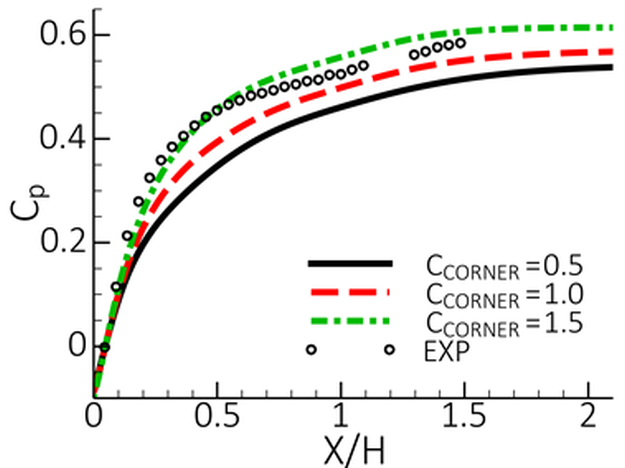
The influence of the model changes on the pressure coefficient, Cp, can be seen in
Figure 12.200: Wall pressure coefficient, , for 3D diffuser for GEKO-1.00 with different
  values.. Note that the current flow is very sensitive and hard to compute, but it
does demonstrate the importance of corner flow separation for technical flows.
values.. Note that the current flow is very sensitive and hard to compute, but it
does demonstrate the importance of corner flow separation for technical flows.
Figure 12.199: Flow topology for 3D diffuser flow shown through streamwise velocity contour at downstream end of diffuser opening section for GEKO-1.00 with different values.
The curvature correction (CC) is an already existing model, which is accessible to all eddy-viscosity models in Fluent. The only change when integrating it with GEKO was that the coefficient CCURV is now also accessible through a User Defined Function (UDF) and can thus be optimized zonally, or even locally.
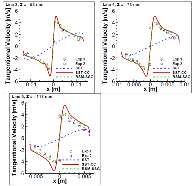
No detailed description of the CC formulation is given, as it is described elsewhere [22]. The effect of the CC can be shown for a hydro-cyclone (see Figure 12.201: Hydrocyclone typical flow structure. Reproduced from Cullivan et al [9].) The flow (typically with particles) enters the domain tangentially through the feed. A strong swirl is generated pushing the particles to the wall and out through the underflow, whereas the cleaned fluid leaves the domain through the overflow. The effect of swirl and rotation cannot be handled by eddy-viscosity models without corrections. The current CC serves this purpose, as can be seen by a comparison of the circumferential velocity profiles for the SST model, the SST-CC and a full Reynolds Stress model (RSM-SSG) in Figure 12.202: Time-averaged profiles of the tangentional velocity in the hydrocyclone. Comparison with the experiments of Hartley [13].. While the model without CC produces mostly a solid-body rotation, the SST-CC model gives results much closer to the experiments and similar to a full Reynolds Stress model (note that at the time of writing, the GEKO model has not been run for this test case. However, the effect of the CC is mostly independent of the underlying model formulation).
![Hydrocyclone typical flow structure. Reproduced from Cullivan et al [].](graphics/image.png)
Figure 12.202: Time-averaged profiles of the tangentional velocity in the hydrocyclone. Comparison with the experiments of Hartley [13].
![Time-averaged profiles of the tangentional velocity in the hydrocyclone. Comparison with the experiments of Hartley [].](graphics/firstimage.png)
The blending function activates the coefficients  /
/ . In order to avoid any
impact on boundary layers, the blending function is designed such that these
parameters have only a minor effect there. In most cases the users will not have to
change the function FGEKO (in Fluent it is called 'Blending Function for GEKO').
However, there are several ways to modify the function in case it is needed.
. In order to avoid any
impact on boundary layers, the blending function is designed such that these
parameters have only a minor effect there. In most cases the users will not have to
change the function FGEKO (in Fluent it is called 'Blending Function for GEKO').
However, there are several ways to modify the function in case it is needed.
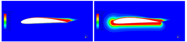
The easiest way is to adjust the coefficients exposed in the GUI. For fully turbulent
flows (no transition model) there is only one coefficient called CBF_TURB (GEKO).
Increasing it will increase the thickness of the near wall 'shielding' and decreasing
it will decrease the 'shielding' from  /
/ inside the boundary layer. This effect
can be seen in Figure 12.203: Effect of CBF_TURB on
inside the boundary layer. This effect
can be seen in Figure 12.203: Effect of CBF_TURB on  for flow around airfoil. Left CBF_TURB=2.0. Right: CBF_TURB=4.0. for the flow around a NACA 4412 airfoil. The lefts side of
the figure shows the default setting (CBF_TURB=2) and the right side the function for
CBF_TURB=4. The thickness of the boundary layer 'shielding' is clearly increased on
the right part of the figure.
for flow around airfoil. Left CBF_TURB=2.0. Right: CBF_TURB=4.0. for the flow around a NACA 4412 airfoil. The lefts side of
the figure shows the default setting (CBF_TURB=2) and the right side the function for
CBF_TURB=4. The thickness of the boundary layer 'shielding' is clearly increased on
the right part of the figure.
There is a second coefficient for this function, which is a bit more involved.
It is introduced to allow protection of the laminar boundary layer from the  /
/ term. This is desirable in case of transition predictions [16], where
otherwise the
term. This is desirable in case of transition predictions [16], where
otherwise the  /
/ term can affect the transition location. For this purpose, a second
coefficient, CBF_LAM (GEKO) is used in case a transition model is selected. The effect is shown
in Figure 12.204: Effect of CBF_LAM on
term can affect the transition location. For this purpose, a second
coefficient, CBF_LAM (GEKO) is used in case a transition model is selected. The effect is shown
in Figure 12.204: Effect of CBF_LAM on  for flow around airfoil. Left CBF_LAM=1.0 (default for turbulent simulations). Right: CBF_LAM=25 (default for transitional simulations). . The left figure shows the turbulent default
(CBF_TURB=2.0, CBF_LAM=1.0 same as Figure 12.203: Effect of CBF_TURB on for flow around airfoil. Left CBF_TURB=2.0. Right: CBF_TURB=4.0. Left) and the right part shows the increase to its default
for transitional simulations (CBF_TURB=2.0 CBF_LAM=25.0). As can be seen from the right part of
Figure 12.203: Effect of CBF_TURB on for flow around airfoil. Left CBF_TURB=2.0. Right: CBF_TURB=4.0., the coefficient CBF_LAM provides increased shielding,
especially in the leading edge region. In case of fully turbulent settings (no transition
model), users can only access CBF_TURB (CBF_LAM=1.0 is fixed by default). The parameter CBF_LAM
becomes available once a transition model is selected. The coefficient CBF_LAM needs to always
satisfy
for flow around airfoil. Left CBF_LAM=1.0 (default for turbulent simulations). Right: CBF_LAM=25 (default for transitional simulations). . The left figure shows the turbulent default
(CBF_TURB=2.0, CBF_LAM=1.0 same as Figure 12.203: Effect of CBF_TURB on for flow around airfoil. Left CBF_TURB=2.0. Right: CBF_TURB=4.0. Left) and the right part shows the increase to its default
for transitional simulations (CBF_TURB=2.0 CBF_LAM=25.0). As can be seen from the right part of
Figure 12.203: Effect of CBF_TURB on for flow around airfoil. Left CBF_TURB=2.0. Right: CBF_TURB=4.0., the coefficient CBF_LAM provides increased shielding,
especially in the leading edge region. In case of fully turbulent settings (no transition
model), users can only access CBF_TURB (CBF_LAM=1.0 is fixed by default). The parameter CBF_LAM
becomes available once a transition model is selected. The coefficient CBF_LAM needs to always
satisfy  .
.
Figure 12.203: Effect of CBF_TURB on for flow around airfoil. Left CBF_TURB=2.0. Right: CBF_TURB=4.0.
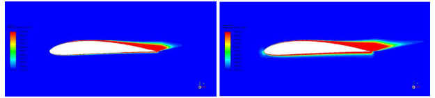
Figure 12.204: Effect of CBF_LAM on for flow around airfoil. Left CBF_LAM=1.0 (default for turbulent simulations). Right: CBF_LAM=25 (default for transitional simulations).
Finally, the function FGEKO can be adjusted through a User Defined Function (UDF).
Users can either over-write the function in the entire domain, or only in certain
parts, as the original function is accessible in the UDF. This could make sense in
areas where free shear flows and boundary layers cannot be easily discerned by the
function itself, especially when  is increased to obtain more mixing in the free
shear flow region.
is increased to obtain more mixing in the free
shear flow region.
An example of such a flow is shown in Figure 12.205: Blending function  for multi-element airfoil. Upper left: Default
  =1.75,
  =
= =0.303. Upper right:
  =3. Bottom left:
  through UDF for a
multi-element airfoil. Assume, the wake of the slat (upstream airfoil) over the main airfoil is
of interest. Assume that the default settings provide not enough mixing in this region, hence an
increased mixing through increases in
through UDF for a
multi-element airfoil. Assume, the wake of the slat (upstream airfoil) over the main airfoil is
of interest. Assume that the default settings provide not enough mixing in this region, hence an
increased mixing through increases in  is desired. This works for moderate increases in
  , but large increases (like
  =3) lead to decreasing efficiency of the
  term. The reason is that through increases in the eddy-viscosity, the blending
function becomes activated also in the wake, due to the proximity of the main airfoil wall. This
is shown in the upper right of Figure 12.205: Blending function for multi-element airfoil. Upper left: Default =1.75, ==0.303. Upper right: =3. Bottom left: through UDF, where one can clearly see the
activation of the blending function in the wake of the slat. To counter such an effect, one can
over-write the blending function. In the current case, a function based on wall-distance was
used as shown in the bottom left of Figure 12.205: Blending function for multi-element airfoil. Upper left: Default =1.75, ==0.303. Upper right: =3. Bottom left: through UDF. Note that this is just a
generic example to demonstrate the issues and no effort was made to optimize the bending
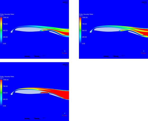
function. The effect of the change in the function
term. The reason is that through increases in the eddy-viscosity, the blending
function becomes activated also in the wake, due to the proximity of the main airfoil wall. This
is shown in the upper right of Figure 12.205: Blending function for multi-element airfoil. Upper left: Default =1.75, ==0.303. Upper right: =3. Bottom left: through UDF, where one can clearly see the
activation of the blending function in the wake of the slat. To counter such an effect, one can
over-write the blending function. In the current case, a function based on wall-distance was
used as shown in the bottom left of Figure 12.205: Blending function for multi-element airfoil. Upper left: Default =1.75, ==0.303. Upper right: =3. Bottom left: through UDF. Note that this is just a
generic example to demonstrate the issues and no effort was made to optimize the bending
function. The effect of the change in the function  is seen in Figure 12.206: Ratio of turbulence to molecular viscosity for multi-element airfoil. Upper left: Default
  =1.75,
  =
= =0.303. Upper right:
  =3. Bottom left:
  through UDF which shows the ratio of turbulence to molecular viscosity for the blending functions and
settings shown in Figure 12.205: Blending function for multi-element airfoil. Upper left: Default =1.75, ==0.303. Upper right: =3. Bottom left: through UDF. Clearly, the ratio increase from the left
(default settings) to the middle picture. However, the increase is moderate. When restricting
the function FGEKO to the immediate boundary layer around the main wing, the effect of
increasing
through UDF which shows the ratio of turbulence to molecular viscosity for the blending functions and
settings shown in Figure 12.205: Blending function for multi-element airfoil. Upper left: Default =1.75, ==0.303. Upper right: =3. Bottom left: through UDF. Clearly, the ratio increase from the left
(default settings) to the middle picture. However, the increase is moderate. When restricting
the function FGEKO to the immediate boundary layer around the main wing, the effect of
increasing  becomes much stronger, resulting in a substantial increase in the viscosity
ratio (Figure 12.206: Ratio of turbulence to molecular viscosity for multi-element airfoil. Upper left: Default =1.75, ==0.303. Upper right: =3. Bottom left: through UDF – right).
becomes much stronger, resulting in a substantial increase in the viscosity
ratio (Figure 12.206: Ratio of turbulence to molecular viscosity for multi-element airfoil. Upper left: Default =1.75, ==0.303. Upper right: =3. Bottom left: through UDF – right).
It needs to be stressed again, that such modifications of  are typically not
required and the flexibility of provided by simply changing coefficients is sufficient in most
cases. However, the discussion shows the versatility of the current GEKO models
implementation.
are typically not
required and the flexibility of provided by simply changing coefficients is sufficient in most
cases. However, the discussion shows the versatility of the current GEKO models
implementation.
Figure 12.205: Blending function for multi-element airfoil. Upper left: Default =1.75, ==0.303. Upper right: =3. Bottom left: through UDF
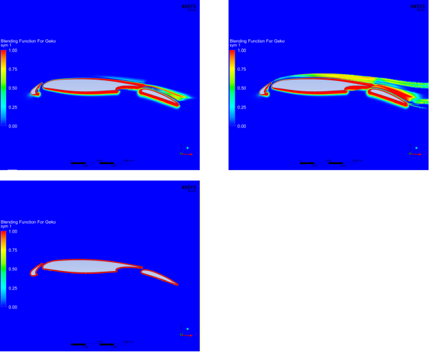
Figure 12.206: Ratio of turbulence to molecular viscosity for multi-element airfoil. Upper left: Default =1.75, ==0.303. Upper right: =3. Bottom left: through UDF
A more dramatic example of how the change in blending function can affect results is given by the flow around a triangular cylinder. The set-up is shown in Figure 12.207: Flow around triangular cylinder [37].
![Flow around triangular cylinder [37]](graphics/image094.png)
The cylinder has an edge length of  , the height of the channel is
  . The
inlet velocity is
. The
inlet velocity is  . The simulation is carried out in steady state mode –
and converges to a steady state solution (which is not always possible with bluff body
flows). The real flow is of course unsteady with strong vortex shedding in addition to
turbulence created unsteadiness. The vector field depicted shows a very large
separation zone downstream of the cylinder, as expected. The simulation was carried out
with GEKO-1.75 (default) under steady-state conditions.
. The simulation is carried out in steady state mode –
and converges to a steady state solution (which is not always possible with bluff body
flows). The real flow is of course unsteady with strong vortex shedding in addition to
turbulence created unsteadiness. The vector field depicted shows a very large
separation zone downstream of the cylinder, as expected. The simulation was carried out
with GEKO-1.75 (default) under steady-state conditions.
In order to test by how much, the re-circulation zone can be reduced, the  coefficient was increased. The results are shown in Figure 12.208: GEKO-1.75 solution under variation of
 ![GEKO-1.75 solution under variation of . Left: Velocity U. Middle: Eddy-viscosity ratio. Right: using built-in function []](graphics/eqbacf164e-f271-4454-bf9a-13f99f7b3c5f.svg) . Left: Velocity U. Middle: Eddy-viscosity ratio. Right:
. Left: Velocity U. Middle: Eddy-viscosity ratio. Right: ![GEKO-1.75 solution under variation of . Left: Velocity U. Middle: Eddy-viscosity ratio. Right: using built-in function []](graphics/eq51de4445-248f-43c1-a34d-9e2aa096154f.svg) using built-in function [28] when using the built-in
version of the
using built-in function [28] when using the built-in
version of the  function. The recirculation (line in middle figure) decreases with
increasing
function. The recirculation (line in middle figure) decreases with
increasing  . However, eventually, the entire separation zone lies within the
 =1 region and no further effect can be achieved by increasing
  .
.
Figure 12.208: GEKO-1.75 solution under variation of . Left: Velocity U. Middle: Eddy-viscosity ratio. Right: using built-in function [28]
![GEKO-1.75 solution under variation of . Left: Velocity U. Middle: Eddy-viscosity ratio. Right: using built-in function []](graphics/image098.png)
The same tests are shown in Figure 12.209: GEKO-1.75 solution under variation of ![GEKO-1.75 solution under variation of . Left: Velocity U Middle: Eddy-viscosity ratio. Right: using UDF-based function []](graphics/eq2329b107-9353-483a-a6e1-29e193ecf2b7.svg) . Left: Velocity U Middle: Eddy-viscosity ratio. Right:
. Left: Velocity U Middle: Eddy-viscosity ratio. Right: ![GEKO-1.75 solution under variation of . Left: Velocity U Middle: Eddy-viscosity ratio. Right: using UDF-based function []](graphics/eq3534fe1b-4af4-4dd1-987e-b3b8a729d320.svg) using UDF-based function [28] but with the help of a UDF-based
using UDF-based function [28] but with the help of a UDF-based  function.
As shown in the right part of the figure,
function.
As shown in the right part of the figure,  is defined only within a given wall
distance as
is defined only within a given wall
distance as  =1 and is switched to free shear flow status outside. This avoids the
restriction of the impact of increasing
=1 and is switched to free shear flow status outside. This avoids the
restriction of the impact of increasing  and allows a further reduction in the
re-circulation zone due to increased mixing.
and allows a further reduction in the
re-circulation zone due to increased mixing.
Figure 12.209: GEKO-1.75 solution under variation of . Left: Velocity U Middle: Eddy-viscosity ratio. Right: using UDF-based function [28]
![GEKO-1.75 solution under variation of . Left: Velocity U Middle: Eddy-viscosity ratio. Right: using UDF-based function []](graphics/image099.png)
The comparison with experimental data along the center-line downstream of the cylinder
is shown for both  variants in Figure 12.210: Center line velocity for triangular cylinder. Left: GEKO-1.75 with built-in
 ![Center line velocity for triangular cylinder. Left: GEKO-1.75 with built-in function. Right: GEKO-1.75 with UDF-based function []](graphics/eq4049615d-2b71-4272-8386-0ffd61c0f48b.svg) function. Right: GEKO-1.75 with UDF-based
function. Right: GEKO-1.75 with UDF-based ![Center line velocity for triangular cylinder. Left: GEKO-1.75 with built-in function. Right: GEKO-1.75 with UDF-based function []](graphics/eqdddd95e0-bb20-4cac-8ae7-9764faf01f77.svg) function [28]. The left part of the figure shows the
solution using the built-in function for
function [28]. The left part of the figure shows the
solution using the built-in function for  and the right part shows the solution
using a wall-distance-based UDF variant (as shown in right part of Figure 12.209: GEKO-1.75 solution under variation of . Left: Velocity U Middle: Eddy-viscosity ratio. Right: using UDF-based function [28]). Clearly,
the UDF based variant allows a much stronger reduction in separation size. It should be
noted that none of the simulations is able to produce the fairly strong backflow
velocity in the re-circulation zone. This should not come as a surprise, as it is
mostly a result of very strong backflow events in the unsteady vortex shedding cycle of
the experiment, which cannot be captured by a steady state solution. Nevertheless, it
is important to observe the much better agreement in flow recovery downstream of the
recirculation zone. In case of more complex arrangements, any additional parts of the
geometry downstream of the triangular cylinder would see a much more realistic
approaching flow field than with the default settings.
and the right part shows the solution
using a wall-distance-based UDF variant (as shown in right part of Figure 12.209: GEKO-1.75 solution under variation of . Left: Velocity U Middle: Eddy-viscosity ratio. Right: using UDF-based function [28]). Clearly,
the UDF based variant allows a much stronger reduction in separation size. It should be
noted that none of the simulations is able to produce the fairly strong backflow
velocity in the re-circulation zone. This should not come as a surprise, as it is
mostly a result of very strong backflow events in the unsteady vortex shedding cycle of
the experiment, which cannot be captured by a steady state solution. Nevertheless, it
is important to observe the much better agreement in flow recovery downstream of the
recirculation zone. In case of more complex arrangements, any additional parts of the
geometry downstream of the triangular cylinder would see a much more realistic
approaching flow field than with the default settings.
Figure 12.210: Center line velocity for triangular cylinder. Left: GEKO-1.75 with built-in function. Right: GEKO-1.75 with UDF-based function [28]
![Center line velocity for triangular cylinder. Left: GEKO-1.75 with built-in function. Right: GEKO-1.75 with UDF-based function []](graphics/image100.5.png)
The realizability coefficient is set to its standard value of  =0.577. The value
should typically not be changed but is accessible for special situations. However, it
was found that limiters can have a strong effect for flows which are severely
under-resolved. An example would be an inlet condition for the velocity field, where
the velocity in the lower half of the inlet has one value and in the upper half
another. At the jump between these two values, the flow is under-resolved and the
coefficient
=0.577. The value
should typically not be changed but is accessible for special situations. However, it
was found that limiters can have a strong effect for flows which are severely
under-resolved. An example would be an inlet condition for the velocity field, where
the velocity in the lower half of the inlet has one value and in the upper half
another. At the jump between these two values, the flow is under-resolved and the
coefficient  could potentially delay the growth of the mixing layer. Note that
for such flows, the production limiter could have a similar effect. If this is the
case, it would be an option to set both limiters to very large values and instead
activate the Kato-Launder limiter.
could potentially delay the growth of the mixing layer. Note that
for such flows, the production limiter could have a similar effect. If this is the
case, it would be an option to set both limiters to very large values and instead
activate the Kato-Launder limiter.
The coefficient CNW_SUB allows for slight re-tuning of the log-layer shift which will also affect the wall shear stress distribution for boundary layers. Increasing its value from CNW_SUB=1.7 will shift the log-layer more into the laminar direction (up) and decrease the wall shear stress.
[5] There are no experimental data for the pressure coefficients for the DU-96-W-180 and DU-97-W-300 airfoils. Only distribution of lift coefficient in wide range of angles of attack are available.