


The following topics are discussed:
The main characteristic of the GEKO model is that it has several free parameters for tuning the model to different flow scenarios. The starting point for the formulation is:
 | (12–114) |
 | (12–115) |
 | (12–116) |
 | (12–117) |
 | (12–118) |
 | (12–119) |
 | (12–120) |
with


The free coefficients of the GEKO model are implemented through the functions
( ,
, ,
,
 )
which can be tuned by the user to achieve different goals in different parts of the
simulation domain. Currently there are six parameters included for that purpose:
)
which can be tuned by the user to achieve different goals in different parts of the
simulation domain. Currently there are six parameters included for that purpose:

Main parameter for adjusting separation prediction for boundary layers
Affects all flows - Increasing
 reduces eddy-viscosity leading
to more sensitivity to adverse pressure gradients for boundary
layers and to lower spreading rates for free shear flows
(compensated by
reduces eddy-viscosity leading
to more sensitivity to adverse pressure gradients for boundary
layers and to lower spreading rates for free shear flows
(compensated by  ).
).

Affects mostly the inner part of wall boundary layers (limited to no impact on free shear flows.
Increasing
 leads to higher wall shear stress and wall heat
transfer rates in non-equilibrium flows.
leads to higher wall shear stress and wall heat
transfer rates in non-equilibrium flows. Effect on non-generic flows (e.g. vortices) moderate but not systematically tested.
Users can mostly use
 = 0.5 (default).

Affects only free shear flows (boundary layer shielded due to function Fblend).
Increasing
 increases spreading rates of free shear flows.
For each value of
 an optimal value of
  exists,
which maintains optimal free shear flows. This value is given
by the correlation
exists,
which maintains optimal free shear flows. This value is given
by the correlation  =
= which is default


Is active in a sub-model of
 (no impact for
  = 0).
= 0).Affects mostly jet flows. Increasing
 while
while  is active,
decreases spreading rate for jets.
is active,
decreases spreading rate for jets. Allows to adjust spreading rate of jet flows while maintaining spreading rate of mixing layer.
Users can mostly use
 = 0.9 (default).
Has no effect in case of
 = 0
= 0

Non-linear stress-strain term to account for secondary flows in corners (e.g. wing-body junctions etc. [17]).

All coefficients (except of  which is of minor importance) can be accessed globally
or locally through User Defined Functions (UDFs), allowing a global or zonal model
optimization.
which is of minor importance) can be accessed globally
or locally through User Defined Functions (UDFs), allowing a global or zonal model
optimization.
The coefficients  and
and  affect boundary layers, whereas
  and
and  are designed
for free shear flows. In order to avoid any influence of
are designed
for free shear flows. In order to avoid any influence of  and
and  onto boundary
layers, a blending function is introduced, which de-activates
onto boundary
layers, a blending function is introduced, which de-activates  and
and  in the
boundary layer. The function is similar to the blending function used in the BSL/SST
model formulation and given by:
in the
boundary layer. The function is similar to the blending function used in the BSL/SST
model formulation and given by:
 | (12–121) |
This function activates the free shear flow parameters as follows:
 | (12–122) |
There are two important aspects. Firstly, the function  =1 inside boundary layers
and
=1 inside boundary layers
and  =0 for free shear flows. Secondly, the parameter
  is a sub-parameter of
 . It only affects the simulation in case
 0.
0.
The free coefficients should be in the range (defaults in parenthesis):
MIN | Parameter | MAX | Default | |||
|---|---|---|---|---|---|---|
0.7 |
|
|
| 2.5 | 1.75 | |
-2.0 |
|
|
| 2.0 | 0.50 | |
0.0 |
|
|
| 1.0... |
| |
0.0 |
|
|
| 1.0 | 0.90 | |
0.0 |
|
|
| 1.5 | 1.00 | |
0.0 |
|
|
| 1.5 | 1.00 |


The greyed values for  are only suggestions. There might be situations where values
higher than 1.0 can be appropriate.
are only suggestions. There might be situations where values
higher than 1.0 can be appropriate.
As mentioned above, for the coefficient  a correlation is provided as default, which
ensures that changes in
a correlation is provided as default, which
ensures that changes in  do not negatively affect free mixing layers:
 | (12–123) |
It is well-known that any conventional two-equation model exhibits build-up of
turbulence in stagnation regions of bluff bodies (like leading edges of airfoils etc.).
The reason lies in the substitution of the eddy-viscosity assumption into the
production term  of the two-equation model. The eddy-viscosity assumption is not
representing the physics correctly in such regions and leads to an over-production of
turbulence kinetic energy, which in turn can lead to excessive eddy-viscosity levels in
these areas. This can have a detrimental effect on the flow over the rest of the
geometry, as the boundary layers starting from the leading edge stagnation point would
be predicted incorrectly. This can cause large errors and even false separation. Such
situations do not only appear in classical stagnation zones of airfoils, but in many
technical flows, where flows hit on a surface or different flow streams collide to form
a stagnation region.
of the two-equation model. The eddy-viscosity assumption is not
representing the physics correctly in such regions and leads to an over-production of
turbulence kinetic energy, which in turn can lead to excessive eddy-viscosity levels in
these areas. This can have a detrimental effect on the flow over the rest of the
geometry, as the boundary layers starting from the leading edge stagnation point would
be predicted incorrectly. This can cause large errors and even false separation. Such
situations do not only appear in classical stagnation zones of airfoils, but in many
technical flows, where flows hit on a surface or different flow streams collide to form
a stagnation region.
There are numerous remedies for that problem. The most widely known is the use of the
so-called Kato-Launder correction [15] whereby the square of the shear strain in  is
replaced by strain times vorticity:
is
replaced by strain times vorticity:
 | (12–124) |
This option is available, albeit typically not by default. It is however activated when using the GEKO model in combination with a model for laminar-turbulent transition, as it prevents even small production rates which can have a significant effect on transitional flows. It should be noted that the Kato-Launder modification can have an effect on flows with rotation and swirl relative to the original model calibration. It also leads to un-physical production in rotating systems as pointed out by Durbin and Reif [11] and should therefore be applied with caution.
An alternative was proposed by Menter [17] in form of a production limiter:
 | (12–125) |
The limiting coefficient can be chosen fairly large (typically  =10), relative to
the equilibrium relation
=10), relative to
the equilibrium relation  . It will therefore not affect any calibrated flow
and still avoids the stagnation build-up and is used as a default option in GEKO (as
in all other
. It will therefore not affect any calibrated flow
and still avoids the stagnation build-up and is used as a default option in GEKO (as
in all other  based models in Ansys CFD).
A more theoretical concept can also be applied by imposing a realizability constraint. Realizability demands e.g. that all normal Reynolds Stress components need to always remain positive (e.g. [11]). This is clearly true from a physical standpoint, but can be violated by eddy-viscosity models (as well as EARSM and RSM). One can argue about how important this constraint is from a practical standpoint, as eddy-viscosity models do not attempt to accurately describe each single Reynolds Stress, but model essentially the principal shear stress. Still, the realizability constraint can, as a side-effect, help to avoid stagnation build up. For eddy-viscosity models it reads:
 | (12–126) |
The realizability limiter has the additional benefit to prevent numerical break-down
in case  approaches zero at any point in the domain. Without the constraint in the
denominator, this would lead to arbitrarily high eddy-viscosities, whereas with the
limiter, such points are typically handled gracefully.
approaches zero at any point in the domain. Without the constraint in the
denominator, this would lead to arbitrarily high eddy-viscosities, whereas with the
limiter, such points are typically handled gracefully.
In the GEKO model the realizability limiter is utilized in addition to the production limiter by default. Users can change the values of both coefficients.
The near wall formulation of a turbulence model has a substantial effect on its
accuracy and its robustness. In addition, modern CFD codes typically feature
so-called  -insensitive wall formulations, which allow the user to obtain sensible
simulations over a wide range of grids with different
-insensitive wall formulations, which allow the user to obtain sensible
simulations over a wide range of grids with different  near wall resolutions.
The GEKO model family was designed by sticking closely to the original  model
formulation – following the argument that the modeled
model
formulation – following the argument that the modeled  is proportional to
 and not to the physical turbulence kinetic energy. The peak observed in the
turbulence kinetic energy in the buffer layer is therefore not modelled, as it
consists mostly of passive motion (no effect on shear stress).
and not to the physical turbulence kinetic energy. The peak observed in the
turbulence kinetic energy in the buffer layer is therefore not modelled, as it
consists mostly of passive motion (no effect on shear stress).
A  -insensitive wall formulation has been developed for the GEKO model (similar to
what is used in the BSL and SST models). It allows the use of the model, on meshes of
arbitrary
-insensitive wall formulation has been developed for the GEKO model (similar to
what is used in the BSL and SST models). It allows the use of the model, on meshes of
arbitrary  values, as long as the
  -value lies in the logarithmic layer of the
boundary layer, and as long as the rest of the boundary layer is resolved with a
sufficient number of cells.
-value lies in the logarithmic layer of the
boundary layer, and as long as the rest of the boundary layer is resolved with a
sufficient number of cells.

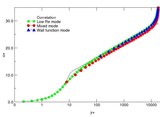
The  -insensitive wall formulation has the advantage that users do not have to select
a wall treatment. The optimal formulation is selected by the formulation based on the
grid provided.
-insensitive wall formulation has the advantage that users do not have to select
a wall treatment. The optimal formulation is selected by the formulation based on the
grid provided.
It is important to counter a widely held belief that  based models require a finer
near wall resolution than say a
based models require a finer
near wall resolution than say a  model with wall functions. This is not correct,
as the
model with wall functions. This is not correct,
as the  -insensitive wall formulation blends to the exact same wall function once the
grid is coarsened.
-insensitive wall formulation blends to the exact same wall function once the
grid is coarsened.
In order to demonstrate the superior behavior of  based models compared with other models, a backstep was computed on a y+~1
mesh. The wall shear stress and Stanton number (heat transfer) distribution downstream of the
step are shown in Figure 12.171: Wall shear stress coefficient,
based models compared with other models, a backstep was computed on a y+~1
mesh. The wall shear stress and Stanton number (heat transfer) distribution downstream of the
step are shown in Figure 12.171: Wall shear stress coefficient, ![Wall shear stress coefficient, (left) and wall heat transfer coefficient, St, (right) for backward-facing step flow [31]](graphics/eq45d2806e-528e-4af0-8075-22dc81b38a6c.svg) (left) and wall heat transfer coefficient, St, (right) for backward-facing step flow [31]. All curves are based on the same high Re
number
(left) and wall heat transfer coefficient, St, (right) for backward-facing step flow [31]. All curves are based on the same high Re
number  model (the GEKO model is set to an exact transformation of
  ). The ML is a low Re number
  model, EWT is a 2-layer formulation [35] and the V2f model is an extension of
 with elliptic blending [12]. While all baseline models are essentially
identical, the differences in near wall formulation results in very large differences between
the results. It is obvious that the GEKO model is closest to the experimental data.
with elliptic blending [12]. While all baseline models are essentially
identical, the differences in near wall formulation results in very large differences between
the results. It is obvious that the GEKO model is closest to the experimental data.
Figure 12.171: Wall shear stress coefficient, (left) and wall heat transfer coefficient, St, (right) for backward-facing step flow [31]
![Wall shear stress coefficient, (left) and wall heat transfer coefficient, St, (right) for backward-facing step flow [31]](graphics/image029.5.png)
In order to clearly characterize the model variant used in an application, it is important to have a unified terminology for the model. It is proposed to just name the coefficients which are not default.
GEKO with
 =1.2,
=1.2,  =1.0,
=1.0,  =1.0,
=1.0,  =0.9 would be termed
GEKO:(
 =1.2,
=1.2,  =1.0,
=1.0,  =1.0).
GEKO with
 =1.5,
=1.5,  =0.0,
=0.0,  =CMixCor,
  =1.0 would be termed
GEKO:(
 =1.5,
=1.5,  =0.0,
=0.0,  =1.0).
Situations where only
 is changed (most frequent case) will just be characterized in short notion:
GEKO with
 =1.5 will be termed GEKO-1.5