


Note: Acoustic Reflectivity settings are available for subsonic inlet boundaries that are based on:
Static Pressure
Total Pressure
Normal Speed / Velocity Components
Mass Flow
For details, see General Non-Reflecting Boundary Conditions.
Specify the magnitude of the resultant normal velocity at the boundary. The value you specify is transferred from the fluid domain normal to each element face on that boundary during the execution of the CFX-Solver.
This option is especially useful for non-planar inlet boundaries (that is, curved surfaces).
If the domain is porous, the speed that you specify is interpreted as true, not superficial.
Specify the Cartesian components of velocity on the inlet boundary. The component values are relative to the selected coordinate frame.
If the domain containing the boundary condition is rotating, then the axis of the cylindrical coordinate system will automatically be set to the rotation axis. You can specify either relative or absolute velocity components by choosing Frame Type:
If the Frame Type is
Rotating, then your velocity components are relative to the local domain rotating frame of reference.If the Frame Type is
Stationary, then your velocity components are relative to the absolute (stationary) frame of reference (at its initial orientation for transient cases).
If the domain is porous, the velocity components that you specify are interpreted as true, not superficial.
Specify the r, theta, z components of velocity on the inlet boundary in cylindrical coordinates. The axis about which the velocity components are specified depends on the domain motion (rotating or stationary) and on whether a local rotation axis is specified with the boundary condition.
If the domain containing the boundary condition is stationary, you must specify an axis in one of two ways:
You can select the axis of the cylindrical coordinate system for the boundary condition (called the Rotation Axis) as an axis of the global coordinate frame, Coord 0.
You can specify Rotation Axis From and Rotation Axis To points. These are the two end points of the axis. The global coordinate system must be used to specify these points. The positive z component of the cylindrical coordinates is in the direction of the vector from the Rotation Axis From point to the Rotation Axis To point.
If the domain containing the boundary condition is rotating, then the axis of the cylindrical coordinate system will automatically be set to the rotation axis. You can specify either relative or absolute velocity components by choosing Frame Type:
If the Frame Type is
Rotating, then your velocity components are relative to the local domain rotating frame of reference.If the Frame Type is
Stationary, then your velocity components are relative to the absolute (stationary) frame of reference (at its initial orientation for transient cases).
If the domain is porous, the velocity components that you specify are interpreted as true, not superficial.
When Mass and Momentum > Option
is set to Mass Flow Rate, you must set Mass
and Momentum > Mass Flow Rate. A
positive value represents mass flow through the boundary in the specified
flow direction. For details, see Flow Direction.
You must also choose one of two settings for Mass Flow Rate Area:
As SpecifiedMass Flow Rate corresponds to the modeled sector, and is applied directly to the boundary. This setting is selected by default.
Total for All SectorsThis setting is available only for single phase cases that have rotational periodicity and that have a rotational periodic interface. If no rotational periodic interface is present,
Total for All Sectorsis identical toAs Specified. For details on interface models with rotational periodicity, see Interface Models.Mass Flow Rate corresponds to the full geometry. The pair of rotational periodic interfaces (or, in the case of multiple pairs existing in the domain, one such pair) is used to calculate the sector angle (the angle that the modeled sector spans in the full geometry). Mass Flow Rate is multiplied by the ratio between the sector angle and 360° before being applied to the boundary.
Note: Only one sector angle is calculated per domain. If you have defined multiple pairs of rotational periodic interfaces in the same domain, and they spanned different sector angles, you should check the CFX-Solver Output file to see which sector angle was used.
If you want to specify the total pressure at an inlet, you can use the
Total Pressure option. You must specify the
Relative Total Pressure and a flow direction. For
details, see Flow Direction.
The boundary mass flow is an implicit result of the flow simulation. This option is available for both single and multiphase simulations. When running multiphase simulations, the boundary condition is applied as if all phases are incompressible. For details, see Multiphase Total Pressure in the CFX-Solver Theory Guide.
This is the same as the Total Pressure condition in a
stationary domain. In a rotating domain, the total pressure is based on
stationary frame conditions.
If you want to specify the static pressure at an inlet, you can use the
Static Pressure option. You must specify the
Relative Static Pressure and a flow direction. For
details, see Flow Direction.
The boundary mass flow is an implicit result of the flow simulation. For multiphase simulations, the static pressure is the same for all phases and the flow direction on a fluid dependent basis.
This setting is less stable than the total pressure condition because it weakly constrains the momentum that passes through the boundary. It is constrained only by transverse stresses. It is therefore a useful condition to obtain a fully developed velocity profile but is also less robust than the total pressure condition.
This option is only available for an inhomogeneous multiphase simulation.
When this option is selected, the Mass and Momentum
information is set on a per fluid basis using Normal
Speed, Cartesian/Cylindrical Velocity
Components or Mass Flow Rate.
If the domain is porous, the velocity components that you specify are interpreted as true, not superficial.
The flow direction can be specified as normal to the boundary, in terms of Cartesian components or in terms of cylindrical direction components. The direction constraint for the normal to boundary option is the same as that for the Normal Speed option.
If the flow direction is set as normal to the boundary, a uniform mass influx is assumed to exist over the entire inlet boundary. Also, if the flow direction is set using Cartesian or cylindrical components, the component normal to the boundary condition is ignored. Again, a uniform mass influx is assumed.
When using cylindrical direction components, a rotation axis must be set for stationary domains and can optionally be set for rotating domains. The axis used follows the same rules as when setting cylindrical velocity components. For details, see Cylindrical Velocity Components.
For static pressure inlets, the flow direction can also be set to
Zero Gradient, which implies that the velocity gradient
perpendicular to the boundary is zero. This is the most appropriate option for
fully developed flow. For best accuracy with this option, the mesh elements
should be close to orthogonal perpendicular to the interface.
You should set reasonable values of either the turbulence intensity, or
k and  at an inlet boundary. Several
options exist for the specification of turbulence quantities at inlets. However,
unless you have absolutely no idea of the turbulence levels in your simulation
(in which case, you can use the
at an inlet boundary. Several
options exist for the specification of turbulence quantities at inlets. However,
unless you have absolutely no idea of the turbulence levels in your simulation
(in which case, you can use the Medium (Intensity =
5%) option), you should use well chosen values of
turbulence intensities and length scales.
Nominal turbulence intensities range from 1% to 5% but will depend on your specific application. The default turbulence intensity value of 0.037 (that is, 3.7%) is sufficient for nominal turbulence through a circular inlet, and is a good estimate in the absence of experimental data. The allowable range of turbulence intensity specification for an inlet boundary is from 0.001 to 0.1 (that is, 0.1% to 10%), corresponding to very low and very high levels of turbulence in the flow, respectively.
If you know roughly the level of incoming turbulence (that is, the intensity),
you can specify this together with an appropriate length scale. For internal
flows, a fraction of the inlet hydraulic diameter is usually a good
approximation for the length scale. If you want to specify values of
k and  directly, then you can approximate incoming levels for internal flow by using
the following relationships:
directly, then you can approximate incoming levels for internal flow by using
the following relationships:
 | (2–1) |
where I is the specified turbulence intensity.  can then
be approximated using:
can then
be approximated using:
 | (2–2) |
where D h is the hydraulic diameter of the inlet. Strictly, these relationships are only applicable for a small inlet to a large domain and should be used with caution. In cases where the hydraulic diameter is not appropriate, and no experimental data is available, you should use uniform profiles for the turbulence quantities, based on mean flow characteristics.
For equally valid related guidelines on choosing a length scale, see Turbulence Length Scale and Hydraulic Diameter in the Fluent User's Guide.
For external flows, such as flow over an airfoil, relationships based on the geometric scale of the inlet boundary may not be appropriate. Therefore, you should consider using a length scale that is based on the size of the object over which flow is moving.
In turbulent simulations, you should also consider the nature of the flow upstream of the region of interest, and determine whether it would increase or decrease the magnitude of the turbulence intensity in the region you want to model.
The options available for turbulence at an inlet are:
The default turbulence intensity of 0.037 (3.7%) is used together
with a computed length scale to approximate inlet values of
k and  . The length scale is calculated
to take into account varying levels of turbulence. In general, the
autocomputed length scale is not suitable for external flows.
. The length scale is calculated
to take into account varying levels of turbulence. In general, the
autocomputed length scale is not suitable for external flows.
This option enables you to specify a value of turbulence intensity but the length scale is still automatically computed. The allowable range of turbulence intensities is restricted to 0.1%-10.0% to correspond to very low and very high levels of turbulence accordingly. In general, the autocomputed length scale is not suitable for external flows.
You can specify the turbulence intensity and length scale directly, from
which values of k and  are
calculated.
are
calculated.

This defines a 5% intensity and a viscosity ratio  equal to 10.
This is the recommended option if you do not have any information about the inlet turbulence.

Use this feature if you want to enter your own values for intensity and viscosity ratio.

You can use this option for fully developed turbulence conditions provided
that you specify the correct fully developed velocity profile. However, for
robustness it is recommended that, instead of using the Zero
Gradient option, you use the fully developed profiles for the
turbulence model variables.
The inlet specification for the energy equation requires a value for the fluid temperature. You should note that ALL temperatures in Ansys CFX are interpreted as absolute values.
Specify the Total Temperature at an inlet. The static temperature is calculated from this value together with the specifications in the Mass and Momentum section.
This is the same as the Total Temperature condition, except for rotating domains. Total temperature is based on stationary frame velocities.
Specify the Total Enthalpy at an inlet. The value of total enthalpy is considered to be the absolute value, including the reference state.
The P1, Discrete Transfer and
Monte Carlo Radiation models enable you to account for
heating of a fluid due to thermal radiation from a boundary. For the
P1 model, consider the case below where a hot wall that
is outside of the fluid domain results in a radiation flux into the domain
through the inlet boundary.
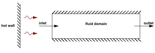
To model the radiation in this case, you would need to specify radiation at
the inlet due to the hot wall using one of the three options described below.
Radiative Flux into the domain for the Monte
Carlo and Discrete Transfer models is
specified on the Sources tab. For details, see Sources (Discrete Transfer and Monte Carlo models).
If this option is selected, you should specify the heat flux through the boundary as a result of thermal radiation.
The radiation intensity is the isotropic mean radiation intensity at the boundary.
This is the effective blackbody temperature of the boundary, for details see External Blackbody Temperature. In the example above, you might set this value to the temperature of the hot wall. In this case, you would be assuming that the hot wall can be treated as a blackbody and that there is no absorption of radiation in the gap between the hot wall and the inlet.
For details, see Local Temperature.
Radiative Flux into the domain for the
Discrete Transfer and Monte
Carlo radiation models is specified via the
Sources tab for the boundary condition in CFX-Pre.
The Monte Carlo model allows directional and isotropic
radiation sources to be specified: the Discrete
Transfer model only allows isotropic radiation
sources.