


Problem Description
This problem is taken from NRC 1677- Volume 2, Problem 1. This problem simulates a 3.5 inch diameter water line extending between two elevations that has two anchors and numerous intermediate supports. Single point response spectrum analysis is performed on the model with base excitation along global X and Y directions.
The input files for this problem are listed below:
| demonstration-problem3-281 Input Listing |
| demonstration-problem3-16-18 Input Listing |
| demonstration_problem3-289-290 Input Listing |
Material Properties:
| Young's modulus = 0.258e8 psi |
| Poisson's ratio = 0.3 |
| Shear modulus = 0.992e7 psi |
| Density = 0.000125 lb-sec2/in4 |
| Set 1: |
| Stiffness of the longitudinal spring-damper element (UX degree of freedom) = 0.2e8 lb/in |
| Stiffness of the longitudinal spring-damper element (UY degree of freedom) = 0.2e8 lb/in |
| Stiffness of the longitudinal spring-damper element (UZ degree of freedom) = 0.2e8 lb/in |
| Set 2: |
| Stiffness of the longitudinal spring-damper element (UX degree of freedom) = 0.2e5 lb/in |
| Stiffness of the longitudinal spring-damper element (UY degree of freedom) = 0.2e5 lb/in |
Geometric Properties:
| Outer diameter = 3.5 inches |
| Wall thickness = 0.216 inches |
| Radius of curvature (for bend pipes) = 48.003 inches |
Loading:
Acceleration response spectrum curve is input on the SV and FREQ commands.
Modeling Notes:
In the piping model using SHELL281 elements, all the rotational degrees of freedom at the end nodes are constrained. In order to simulate the same boundary conditions with pipe elements, the end elements are modeled with ELBOW290 elements. In addition to constraining the nodal degrees of freedom, the ELBOW290 element can also constrain the pipe cross-sections that are not possible with PIPE289 elements, such as warping, ovalization, radial expansion, and shell normal rotations. CONTA175 and TARGE170 elements are used to establish contact between spring-damper elements (COMBIN14) and shell elements (SHELL281).
Results
Results Comparison
Table 1.5: Frequencies Obtained from Modal Solution
| Mode | Results from SHELL281 (A) | Results from PIPE18 and PIPE16 (B) | Results from ELBOW290 (C) | Ratio between A and B | Ratio between A and C |
|---|---|---|---|---|---|
| 1 | 5.989 | 6.047 | 6.113 | 0.990 | 0.979 |
| 2 | 6.230 | 6.269 | 6.353 | 0.993 | 0.980 |
| 3 | 7.893 | 7.759 | 7.766 | 1.017 | 1.016 |
| 4 | 8.800 | 8.922 | 8.793 | 0.986 | 1.000 |
| 5 | 12.259 | 12.441 | 12.185 | 0.985 | 1.000 |
| 6 | 12.758 | 12.830 | 12.627 | 0.994 | 1.010 |
| 7 | 13.917 | 14.297 | 13.956 | 0.973 | 0.997 |
| 8 | 15.363 | 15.484 | 14.866 | 0.992 | 1.033 |
| 9 | 16.096 | 16.369 | 15.987 | 0.983 | 1.006 |
| 10 | 18.218 | 18.540 | 18.061 | 0.982 | 1.008 |
| 11 | 18.888 | 19.496 | 18.921 | 0.968 | 0.998 |
| 12 | 21.943 | 23.223 | 21.609 | 0.944 | 1.015 |
| 13 | 22.973 | 24.080 | 22.958 | 0.954 | 1.000 |
| 14 | 25.390 | 32.634 | 24.942 | 0.778 | 1.017 |
| 15 | 31.411 | 33.749 | 31.874 | 0.930 | 0.985 |
Conclusion
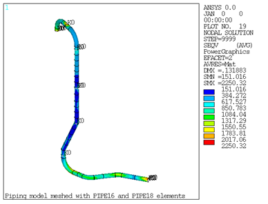
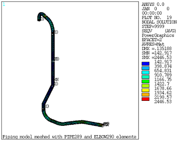
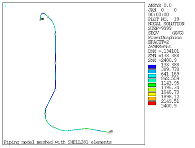
The result comparison table and figures Figure 1.7: Nodal Equivalent Stress Plot from PIPE16/PIPE18 Elements, Figure 1.8: Nodal Equivalent Stress Plot from PIPE289/ELBOW290 Elements, and Figure 1.9: Nodal Equivalent Stress Plot from SHELL281 Elements show that the results obtained from modal and spectrum analyses with PIPE289 and ELBOW290 elements closely match with the results obtained from SHELL281 elements. The higher modes computed from PIPE16 and PIPE18 elements are off by more than 5% when compared with SHELL281 elements. Since only the lower modes are contributing to the spectrum solution, the results obtained from spectrum solution with PIPE16 and PIPE18 elements, PIPE289 and ELBOW290 elements, and SHELL281 elements are all relatively close.