1.4. Demonstration Problem 2

Problem Description

A simple piping model made up of straight and bend pipe elements between two fixed anchors is solved. This problem is similar to the problem specified in NRC1677-Volume 1, Problem 1. Single point response spectrum analysis is performed on the model with base excitation along global X, Y and Z directions.

The input files for this problem are listed below:

demonstration-problem2-290 Input Listing

demonstration-problem2-281 Input Listing

demonstration-problem2-16-18 Input Listing

Material Properties:

Young's modulus = 24e6 psi

Poisson's ratio = 0.3

Density = 0.000125 lb-sec²/in⁴

Geometric Properties:

Outer diameter = 10.932 inches

Wall thickness = 0.241 inches

Radius of curvature (for bend pipes) = 36.30 inches

Loading:

Acceleration response spectrum curve is input on the SV and FREQ commands.

Modeling Notes:

When modeling the piping problem with current technology elements, the straight elements are also modeled using ELBOW290 elements in order to better capture the ovalization from the curved pipe elements to straight pipe elements.

Results

Figure 1.4: Nodal Equivalent Stress Plot Obtained from PIPE16 and PIPE18 Elements

Figure 1.5: Nodal Equivalent Stress Plot Obtained from ELBOW290 Elements

Figure 1.6: Nodal Equivalent Stress Plot Obtained from SHELL281 Elements

Results Comparison

Table 1.3: Frequencies Obtained from Modal Solution

Mode	Results from SHELL281 (A)	Results from PIPE18 and PIPE16 (B)	Results from ELBOW290 (C)	Ratio between A and B	Ratio between A and C
1	45.457	44.673	45.460	1.017	0.999
2	83.403	80.632	83.454	1.034	0.999
3	108.235	103.566	108.532	1.045	0.997
4	202.668	193.109	202.808	1.049	0.999
5	219.772	210.178	219.878	1.045	0.999
6	338.843	329.211	338.765	1.029	1.000
7	344.744	336.523	345.216	1.024	0.998
8	431.890	457.355	431.528	0.944	1.000
9	441.304	466.377	440.802	0.946	1.000
10	491.536	693.369	491.493	0.708	1.000
11	491.876	745.125	491.838	0.660	1.000
12	528.549	763.789	528.446	0.692	1.000
13	563.018	801.945	562.924	0.702	1.000
14	563.899	932.173	563.795	0.604	1.000
15	593.071	947.206	592.365	0.626	1.000

Table 1.4: Displacements and Stresses Obtained from Spectrum Solution

Result Quantities	Results from SHELL281 (A)	Results from PIPE18 and PIPE16 (B)	Results from ELBOW290 (C)	Ratio between A and B	Ratio between A and C
Maximum displacement Vector Sum	5.65 x 10^-3	5.72 x 10^-3	5.65 x 10^-3	1.106	1.000
Maximum equivalent stress	147.522	147.736	160.106	1.024	0.921

Conclusion

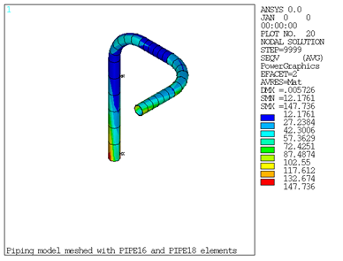
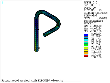
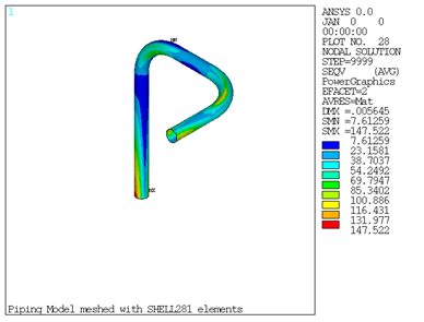
The result comparison table and Figure 1.4: Nodal Equivalent Stress Plot Obtained from PIPE16 and PIPE18 Elements, Figure 1.5: Nodal Equivalent Stress Plot Obtained from ELBOW290 Elements, and Figure 1.6: Nodal Equivalent Stress Plot Obtained from SHELL281 Elements show that the results obtained from modal and spectrum analyses with ELBOW290 elements closely match with the results obtained from SHELL281 elements. The higher modes computed from PIPE16 and PIPE18 elements are off by more than 30% when compared with SHELL281 elements. Since only the lower modes contribute to the spectrum solution, the results obtained from spectrum solution with PIPE16 and PIPE18 elements and the results obtained withELBOW290 and SHELL281 elements are all relatively close.