


The tire-performance simulation is performed in multiple load steps, beginning with the 2D axisymmetric model through the full 3D model. The boundary conditions and loadings are described for the each load step.
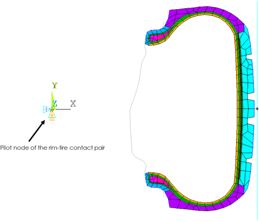
In the 2D axisymmetric model, the rigid rim surface is modeled at the beginning such that it is already at its final position with respect to the tire. It remains fixed by constraining the pilot node of the rim-tire contact pair in all directions:
Alternatively, rim mounting can also be performed by moving the rigid rim surfaces towards the tire. In that case, two separate rigid-rim surfaces are created (one for each end to have contact with the 2D tire cross-section) and pushed towards tire during rim mounting analysis. In this example problem, however, only one rigid rim surface is created at its final position with respect to the tire.
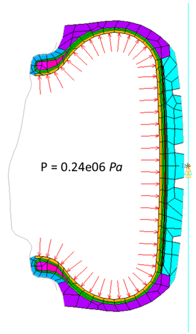
In the second load step (inflation analysis), air pressure is applied on the inner surface of the tire:
Following the rim-mounting and inflation analyses, the 2D axisymmetric tire model is extruded into a 3D model (EEXTRUDE).
All contact pairs, loads, and results are transferred from the 2D axisymmetric model to the 3D model automatically (MAP2DTO3D) and the simulation continues on the 3D tire model for footprint analysis.
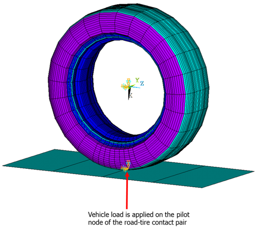
During footprint analysis, contact between the road and the tire is established and the vehicle load is transferred to the tire via the pilot node of the road-tire contact pair:
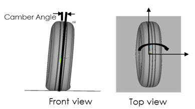
A non-zero camber angle can be added by rotating the rigid road surface appropriately. Camber is the angle between the center line of the wheel and the perpendicular to the road, viewed from the front of the tire:
Following the footprint analysis, a few steady-state rolling analyses are performed to determine various steady-state rolling solutions (including free rolling, braking, and traction for a fixed translational velocity). In the first steady-state rolling analysis, the translational and rotational velocities are applied such that the tire is in a braking condition:
Example 57.3: Applying Translational and Rotational Velocities (3D Tire Model)
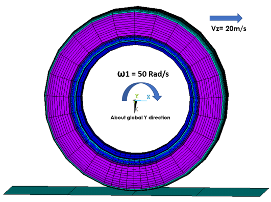
! SSTATE command applies spin and translation velocities.
! “Etire” is an element component defined earlier; it consists
!    of all elements in the 3D tire model.
! The axis of spin is defined via the SSTATE command.
time,5
sstate,define,Etire,spin,50,points,0,0,0,0,1,0
sstate,define,Etire,Translate,,,20
sstate,list
For a given translation velocity, the spin at which there is no longitudinal force along the operational direction of the tire, or no torque acting on the tire, is called the free-rolling spin.
To determine the free-rolling spin, two steady-state rolling analyses are performed (in a separate run), where the translational velocity V remains constant and the rotational velocity increases from ω1 to ω2. (For details, see the free_rolling_analysis.dat input file.)
The ω1 to ω2 values are estimated based on the original and deformed radii of the tire and the given translational velocity. The ω1 and ω2 values are chosen such that the free-rolling spin lies between them.
Example 57.4: Determining the Free-Rolling Spin (3D Tire Model)
This operation is performed in a separate run (as shown in the free_rolling_analysis.dat input file.)
The values ω1 = 50 rad/s and ω2 = 70 rad/s are used, with a translational velocity V = 20 m/s:
! First steady-state rolling analysis, where
!    ω1 = 50rad/s and V = 20m/s
time,5
sstate,define,Etire,spin,50,points,0,0,0,0,1,0
sstate,define,Etire,Translate,,,20
sstate,list
solve

! Second steady-state rolling analysis, where
!    ω2 = 70rad/s and V = 20m/s
time,6
sstate,define,Etire,spin,70,points,0,0,0,0,1,0
sstate,define,Etire,Translate,,,20
sstate,list
solve
After determining the free-rolling spin via a separate run as described above, a second steady-state rolling analysis using the free-rolling spin and the given translational velocity V determine the free-rolling state.
Example 57.5: Establishing the Free-Rolling State (3D Tire Model)
Zero longitudinal force (free rolling) is nearly observed at ωs = 64.1 rad/s, so a second steady-state rolling analysis is performed as follows:
! Second steady-state rolling analysis, where
!     ωs = 64.1 rad/s and V = 20m/s
time,6
sstate,define,Etire,spin,64.1,points,0,0,0,0,1,0
sstate,define,Etire,Translate,,,20
sstate,list
solve
After achieving a free-rolling state, a third steady-state rolling analysis is performed with different slip angles to calculate the cornering force, the lateral force on the tire caused by the vehicle during cornering (making a turn).
At low slip angles, the cornering force is proportional to the slip angleα, the angle between the travel direction of the vehicle and the direction toward which the rolling tire is pointing:
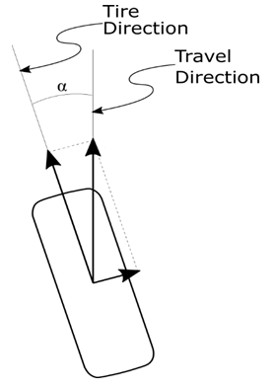
A non-zero slip angle is defined by applying the equivalent lateral velocity component to the tire.
Example 57.6: Defining a Non-Zero Slip Angle
! Translation velocity (Vz) = 20m/s with 0º slip angle,
!     so Vy = 0
! For a 10º slip angle: Vy = 20*Sin(10) and Vz = 20*Cos(10)

time,7
sstate,define,Etire,spin,64.1,points,0,0,0,0,1,0    ! Free rolling
sstate,define,Etire,Translate,,3.473,19.696