


The PSD analysis occurs in three steps:
A modal analysis is performed using the Block Lanczos eigensolver, which is well suited for extracting a medium number of modes (a few hundred) from a moderate-sized model (< 50K DOFs in this case).
Because no element results are needed, only nodal solutions (nodal displacements and rotations) are requested.
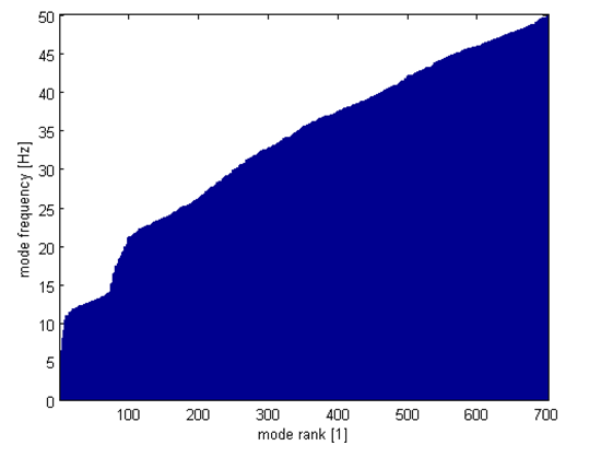
As a general rule, plate-type structures exhibit constant modal density in the medium frequency range. As shown in the following figure, the number of modes within a given frequency range is approximately constant above 22 Hz:
The following input fragment shows the analysis steps involved:
/solu

antype,modal               ! Perform modal solve
modopt,lanb,150,-1.0,50    ! Use Block Lanczos eigensolver to extract 150
                           ! modes with begin frequency FREQB = -1 Hz and with end frequency, FREQE = 50 Hz
outres,all,none
outres,nsol,all            ! Only nodal solution data written to the database
solve
finish

/com, Modes selection based on mode coefficients (ModSelMethod=MODC)
/solu
antype,modal,restart
mxpand,150,,,NO,,,modc     ! Expand all modes and do not evaluate element results
outres,all,none
outres,nsol,all
solve
fini
PSD analyses are performed on the NI using:
Fully coherent input motion with no wave passage effect.
Partial coherent input motion with no wave passage effect.
Partial coherent input motion with wave passage effect.
In each analysis type, the same ground input motion is considered.
For each region (elementary excitation), a unit nodal displacement is input (D), and then modal participation factors are evaluated (PFACT). This is most easily achieved by using an APDL do-loop.
Elementary excitation must be defined for each region using PSD tables. The magnitude-vs.- frequency data can be input with a PSD table (via PSDFRQ, which defines the frequency points of an input spectrum, and PSDVAL, which defines the PSD values of an input spectrum). The PSD curve as defined in Figure 34.4: Ground Motion Power Spectral Density (Acceleration PSD) must be used as an input spectrum. Additionally, the input motion has a unit of acceleration (defined via PSDUNIT).
For cross excitations, PSD co-spectral values are obtained by multiplying the original (direct) PSD values with the plane-wave coherence value, as defined in Figure 34.5: EPRI-TR 1014101 -- Plane Wave Coherency Model for Horizontal Direction, frequency by frequency (COVAL).
For cases where wave-passage effects must be considered, cross PSDs have both a real part (defined via COVAL) and an imaginary part (defined via QDVAL). Both terms are equal to the previous cross-PSD value multiplied by a phasor of unit amplitude, and have an argument equal to the phase shift between the two locations considered. The relationship can be expressed as:[2]

where PSDWavePassage is the co-spectral values of cross PSDs with wave-passage effect, PSDPlaneWave is the spectral values of cross PSDs with no wave-passage effect, and dij is the distance between the two locations i and j.
The distance dij depends on whether the incoherency or the wave-passage effects are being considered:
For incoherency, dij is the Euclidian distance between the two locations (that is, the conventional distance).
For wave-passage effects, dij is the distance along the propagation (orientation) vector. It is the dot product of the vector dij.N, where dij is the vector between nodes i and j, and N is the unitary orientation vector defining the propagation direction).
For simplicity, wave-propagation along the global X-axis is assumed.
Because the absolute acceleration result is the only quantity of interest, only this single calculation is requested (PSDRES).
The response PSD of absolute acceleration quantity is calculated in the POST26 postprocessor (RPSD) and plotted on log-log scale to derive the frequency-by-frequency reduction ratio, as shown in Figure 34.9: PSD Reduction Due to Incoherency and Wave-Passage Effects.