For the thermal analysis using the layered option, the results for the reinforcing ring are shown in the following three figures. It is important to note the layered analysis solution within each layer. For example, the peak TEMP gradient may occur in layer 2, while the peak Von Mises stress may occur in layer 3.
An additional complication to consider when postprocessing elements with layers, is that while regular postprocessing commands can be used, the results will be based on the corner node values, and the values within each layer will be ignored. For example, the PLNSOL,TEMP command will create a contour plot based on the 8 nodes of the element, but it does not reveal how the temperature varies within the 4 layers. To postprocess layer by layer, activate each individual layer, then issue the relevant postprocessing command.
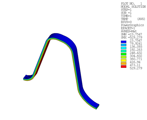
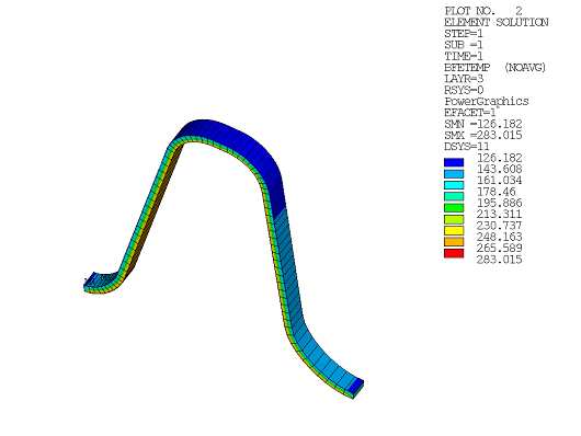
The TEMP in layer 3 of the reinforcing ring is shown in Figure 29.13: Layer 3 Temperature Results. You can generate this by issuing the following command in /POST1:
Layer,3				!activate the layer for postprocessing
presol,bfe,temp	! plot the element stored layer temp
You can also force the layer TEMP onto the 8 corner nodes of the element and then contour the element solution (LAYER). This ensures that the element solution plotted is the actual layer solution in the figure.
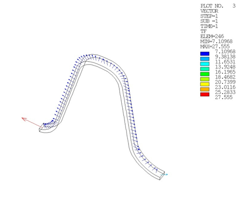
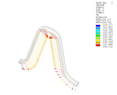
To view the layer heat flux and temp gradient issue the PLESOL command after the LAYER command.
By default the layer value is 0. This implies that the postprocessed quantities are top of top layer and bottom of bottom layer.
The following figures show the displacement solution for the four analyses of the reinforcing ring. These are all node-based plots. The maximum displacement in all cases occurs where the reinforcing ring is bonded to the nozzle body.
The displacement solution for the layered cases do not vary significantly. As a result, using homogeneous or layered thermal loading for the layered mechanical problem does not appear to have a significant effect. A similar conclusion can be drawn for the displacement solution of the homogeneous cases; however, the same conclusion may not be valid for stresses. Do not draw general conclusions based on this model; instead, analyze each model based on its loading conditions and assumptions.

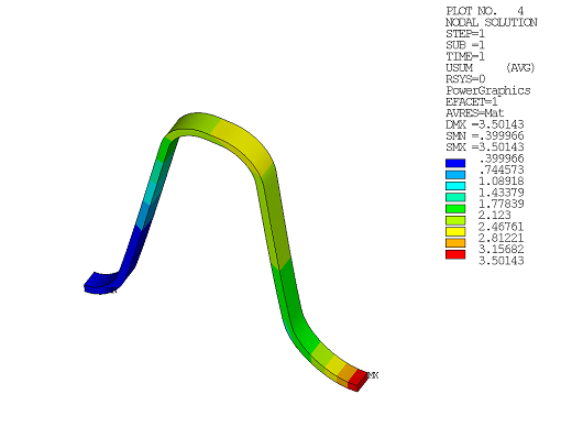
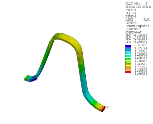
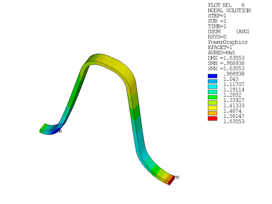
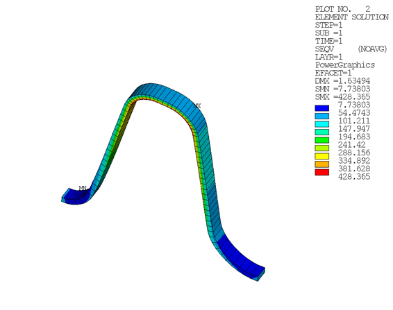
Figure 29.18: Layer 1 Equivalent Stresses shows the equivalent stresses in layer 1. The figure shows that stresses do not peak near the bonded region for layer 1 as might be expected. This underscores the need to analyze the solution layer by layer rather than element by element. Consider changing the ring shape, material, number of layers, or layer orientations to shift the peak stresses to acceptable levels.
When the equivalent stresses in layer 2, 3, and 4 are plotted, the location of peak stresses noticeably shifts. This underscores the need to study each layer carefully and refrain from drawing immediate conclusions about other layers. For example, peak stresses in layer 4 shift to the bonded region, which could not have been predicted from the layer 1 solution alone.