


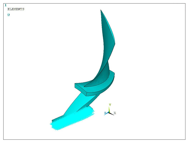
Fixed-support conditions are applied near the disk portion of the cyclic-sector fan blade model, as shown in the following figure:
The following loads are considered for the cyclic symmetry analyses:
Centrifugal loads caused by rotational velocity
Thermal loads due to the difference in reference and operating temperature
Unsteady flow pressure applied on the fan blade (imported from CFX)
The rotational velocity (CGOMGA,0,0,1680) is applied along the global Z-axis. The bladed disk is modeled with a coefficient of thermal expansion of 1.2 x 10⁻⁵ °C-1. The reference temperature is held at 22 °C and an operating temperature of 50 °C is applied on all nodes of the model to generate the thermal load vector.
The thermal load vector generated from the base static solve can be ignored in the subsequent analysis (THEXPAND).
The unsteady flow pressures, which are imported from Ansys CFX, are generated for EO = 2 engine order excitation at a rotational frequency of 534.76 Hz. These pressure data are then mapped to the structural rotor fan blade model in Ansys Mechanical APDL using its mapping capabilities via the /MAP processor.
The following example input shows the steps involved in this mapping procedure:
/map                                   ! Mapping processor
target, nbf1                           ! Specifies target nodes for mapping pressures onto
                                       ! surface effect elements
FTYPE, cfxtbr,1                        ! Specifies file and pressure type for the
                                       ! subsequent import of source points and pressures
READ,CFX_ExportResults_FT_10P_EO2.csv' ! Read coordinate and pressure data from a file

allsel,all,all
csys,0

/show,jpeg,rev
plgeom                                 ! Plots source and target geometries
MAP,,2,,1,                             ! Map pressures from source points to target surface elements
plmap,target                           ! Plot target and source pressure
plmap,target,,,1
/show,close
WRITEMAP,'mapped_on_cyclic_model.dat'  ! Write interpolated pressure
                                       ! data to a file
finish
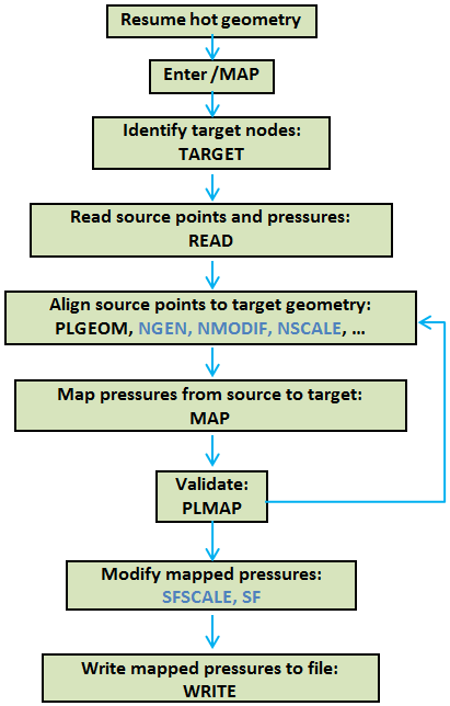
To illustrate the step-by-step mapping procedure, the complete workflow in Mechanical APDL is shown below:
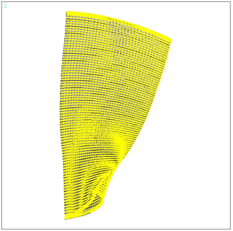
Using the PLGEOM command, the target and source geometries can be plotted as shown:
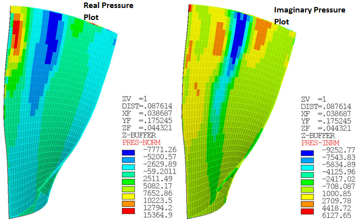
The real and imaginary components of mapped target pressure are plotted using the PLMAP command, as shown:
The procedure for computing aerodynamic coefficients (stiffness and damping terms) for each interblade phase angle is described in Aero Coupling. The AEROCOEFF command uses unsteady pressures obtained from a CFD flutter analysis to compute an aerodynamic coefficient array. This aerodynamic coefficient array is compatible with the CYCFREQ,AERO command. If all interblade phase angles are not available from the CFD computation, the coefficients can be interpolated between nodal diameters and inserted into the aerodynamic coefficient array.
In the case of a mistuned bladed disk, blades are subjected to engine order (EO) excitation. Engine order excitation is the effective traveling wave excitation that a bladed disk experiences as it passes through disturbances in the flow-field for each revolution. For example, one disturbance in the flow field results in an EO = 1 excitation; two disturbances in the flow field result in an EO = 2 excitation.
In Mechanical APDL, the engine order excitation is applied using the
CYCFREQ command with Option = EO.
Internally, the program computes the aliased engine order, including its sign. The
aliased engine order  is determined from the input engine order
  as follows:
Table 45.1: Aliased Engine Order (Excited Harmonic Index)
| Engine Order C | Aliased Engine Order
 | |
|---|---|---|
| N Even | N Odd | |
| C ≤ N / 2 | C ≤ (N - 1) / 2 | C |
| N / 2 < C ≤ N - 1 | 2(N + 1) ≤ C ≤ N | N - C |
| N ≤ C ≤ 3N / 2 | N ≤ C ≤ (3N - 1) / 2 | C - N |
| 3N / 2 ≤ C ≤ 2N | (3N +1) / 2 ≤ C ≤ 2N | 2N - C |
| … | … | … |
where N = number of sectors.
For the case of mistuned forced-response analysis, the forcing/excitation frequency expressed in terms of EO is as follows:

where  is in Hz and
  is in RPM.
The excitation frequency is specified with the HARFRQ command.
In general, mistuning in bladed disks is typically modeled as small, random perturbations to the stiffness of the blade DOF. The deviation in stiffness for blade n is expressed as follows:

where  is the mistuning parameter for blade n.
The mistuning parameters are provided in an array parameter of size N × 1, where
N is the number of blades. These mistuning parameters are defined using the
CYCFREQ command with Option = MIST and
Value1 = K.
For the perturbed mode-superposition harmonic analysis, the unsteady flow pressures applied as per the engine order excitation on the fan blade are treated as a harmonically varying load.