In most cases, a linear buckling analysis provides only an upper limit to the buckling behavior of an actual structure. It is generally preferable, therefore, to perform a nonlinear buckling analysis, which can account for the influence of nonlinear material behavior and large-deflection response.
The following analysis and solution-control topics are available:
The method for obtaining the nonlinear buckling and collapse of the ring-stiffened cylinder is based on the following sequence of actions:
This preliminary analysis predicts the theoretical buckling pressure of the ideal linear elastic structure (perfect cylinder) and the buckled mode shapes used in the next step to generate the imperfections. It is also an efficient way to check the completeness and correctness of modeling.
To run the linear buckling analysis, a static solution with prestress effects must be obtained, followed by the eigenvalue buckling solution using the Block Lanczos method and mode expansion, as shown in the following example input:
/solu
pstres,on                    ! Activate the prestress option
solve
finish
 /solu
outres,all,all
antype,buckle                ! Buckling analysis
bucopt,lanb,10,              ! Mode extraction is Block Lanczos
mxpand,10                    ! Expand mode shapes
solve
finish
If a structure is perfectly symmetric (that is, its geometry--including the mesh patterns--and loading are both symmetric), nonsymmetric buckling does not occur numerically, and a nonlinear buckling analysis fails because nonsymmetric buckling responses cannot be triggered.
In this problem, the geometry, elements, and pressure are all axisymmetric. It is not possible, therefore, to simulate nonaxisymmetric buckling with the initial model. To overcome this problem, small geometric imperfections (similar to those caused by manufacturing a real structure) must be introduced to trigger the buckling responses.
Although small perturbation loads can also be introduced to serve the same purpose, it is not an ideal method because it is difficult to determine how large the loads should be and where to apply them. Also, a perturbation load that is too large can change the problem completely.
The geometric imperfections can be generated either in the shape of the buckling mode or in a given shape with a random amplitude:
The imperfections in the buckling mode shapes are obtained by running a preliminary linear buckling analysis, then updating the geometry of the finite-element model to the deformed configuration. This technique is done by adding the displacements of the mode shapes reduced by a scaling factor. It is safe to add a few mode shapes to avoid any bias in the imperfections.
Introduce pseudo-random imperfections by modifying the coordinates of the nodes with a random number (using the RAND parametric function).
The imperfection magnitudes are generally dependent on the geometry and should be in the same range as the manufacturing tolerance (typically less than one percent) so that they do not change the problem during analysis.
For this problem, the imperfections are added as a sum of the first 10 modes shapes extracted in the preliminary buckling analysis. (While random imperfections can also be used, their disadvantage is that they cannot be repeated; therefore, the results would differ each time the analysis is run.)
Because the radius of the cylinder is 355.69 mm and the maximum displacement of a mode shape is 1 mm, a factor of 0.1 is applied when updating the geometry with mode shapes. The factor assumes the manufacturing tolerance of the radius to be on the order of 0.1. The following input example shows how the imperfections are added:
/prep7
*do,i,1,10
upgeom,0.1,1,i,buckling,rst       ! Add imperfections as a tenth of each mode shape
*enddo
finish
The nonlinear buckling analysis is a static analysis performed after adding imperfections with large deflection active (NLGEOM,ON), extended to a point where the stiffened cylinder can reach its limit load.
To perform the analysis, the load must be allowed to increase using very small time increments so that the expected critical buckling load can be predicted accurately.
The following example input runs the nonlinear buckling analysis:
/solu                           ! Run static analysis
antype,static
nlgeom,on                       ! Specify large deflection
pred,off                        ! No prediction occurs
time,1
nsubst,100,500,10               ! Minimum time increment is 2e-3
rescontrol,define,all,1         ! Write all files for multiframe restart
outres,all,all                  ! Write all solution items to the database
solve
finish
Some convergence difficulty at or after buckling is expected, so is useful to have all restart files available for resuming the analysis with nonlinear stabilization. It is best to have the restart files at each substep (RESCONTROL,DEFINE,ALL,1)--or at least for every few substeps--as it is virtually impossible to know for certain when the buckling is initiated and therefore when to activate the stabilization via the restart.
An unconverged solution of the nonlinear static analysis could mean that buckling has occurred, but that is not always the case. The buckling begins to occur before the deformations become very large, when the structure appears to be undeformed or only slightly deformed.
Buckling initiation is difficult to detect by visual inspection but can be observed by plotting a load-displacement curve or by a monitor file inspection. To detect the moment of buckling initiation, carefully study the monitor file at this stage, as shown in this figure:
From the monitor file, several observations can be made to help determine if buckling has started to occur and at what time, as follows:
Difficulties in convergence occur. The program bisects the load-step increment and attempts a new solution at a smaller load
The maximum displacement monitored has an instantaneous change in value. This is a good indicator of large displacement for a smaller load increment specific to buckling.
The maximum displacement monitored has an instantaneous change in sign. This is another good indication that buckling has begun to occur.
In this example, the change in time (or load) increment, and displacement value, occurs between substeps 10 and 11, which corresponds to TIME = 0.51781 and TIME = 0.53806 and to a pressure between 0.124 MPa and 0.129 MPa. It is therefore very likely that buckling occurred at this time; to be sure, the analysis is continued. The goal is to verify the assessment made at this stage by obtaining the load-displacement behavior over a larger range.
If the convergence difficulty is caused by buckling, resuming the analysis means starting a post-buckling analysis. Because the post-buckling state is unstable, special techniques are necessary to compensate. In a static analysis, nonlinear stabilization is the best option. When local buckling or time-dependent material exists, it is the only option.
A substep experiencing convergence difficulty in the initial run (13 in this case) should generally be avoided as the substep from which to restart; therefore, to continue with a post-buckling analysis, stabilization is activated from substep 10. If convergence occurs at this substep, and assuming minimal stabilization energy, this solution can be accepted.
The following example input runs the post-buckling analysis:
/solu                                   ! Run static analysis
antype,,restart,1,10                    ! Perform multiframe restart at substep 10
nsubst,100,10000,10
stabilize,constant,energy,0.000143      ! Use energy method with constant option
solve
finish
If convergence does not occur, an earlier substep should be tried.
Two methods are available for controlling the stabilization force:
Selecting which method to use, and then choosing the right value for the energy or damping factor, are not trivial decisions. The best option and value to use depends on the type of instability, the type and size of the elements used in the model, and the end time and number of substeps used for the load step. In most cases, the decision is based on a trial-and-error correction process. The goal is to achieve convergence with the smallest stabilization force, which can be controlled in turn by either an energy ratio or damping factor.
For more information, see Using Nonlinear Stabilization in the Structural Analysis Guide.
The following topics describe the nonlinear stabilization methods tried in the ring-stiffened cylinder problem:
The first trial is typically done using the energy option because:
It has a specific range of values that can be used (between 0 and 1), and
After running, it calculates a damping factor at the beginning of the next substep, providing a reference value for the damping factors that can be used (if damping is chosen as the stabilization method).
The first energy value tried provided a damping factor of 0.1e-2, which helped convergence but without producing significant buckling. The damping values were then gradually reduced to 0.1e-5 and, even though in each case convergence was achieved, the collapse due to buckling did not occur. A value of 0.1e-6 did not result in convergence and the trials for applying the damping factor method ceased.
The observed is due to the localized phenomena inherent in this problem. When damping is applied, the specified value is used for all elements. When the applied damping value is too large, too much stabilization force is applied to the structure, so the system is too stiff and converges easily without much deformation. Conversely, when the applied damping is too small, the unstable elements do not benefit from sufficient stabilization forces, so the solution diverges.
The conclusion is that the damping option is not ideal for problems involving significant local buckling.
Because this problem is characterized by local rather than global instabilities, the energy method for stabilization is more helpful. The energy method uses different damping values for different elements, so elements with large instability have higher damping values and elements with little instability have small damping values. It is therefore possible to compensate for the instability without the system becoming too stiff.
After determining that this problem should use stabilization via the energy method, several trials were performed using energy ratios in a range from 0.001 to 0.0001. The trials showed that larger energy ratios result in convergence, but with no significant deformation and excessive stabilization energy, and smaller energy ratios result in no convergence.
The smallest stabilization energy ratio to offer convergence was found to be 0.000143. With that value, the analysis converges and the full loading is reached, while significant buckling is observed and global stabilization energy is kept at the lowest possible level.
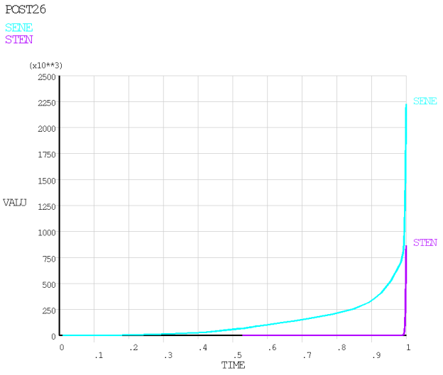
The following figure shows a time-history plot of the stiffness and stabilization energies: