


Some tasks performed by the Ansys-Adams Interface involve substantial "behind-the-scenes" work. Two tasks in particular fall in this category: the creation of the modal neutral file (Jobname.mnf) and the addition of weak springs via the WSPRINGS command.
The following sections provide details concerning how Mechanical APDL performs those tasks.
The algorithm used to create the modal neutral file (.mnf) is based on a formulation called component mode synthesis (also known as dynamic substructuring). Adams uses the approach of Craig Bampton with some slight modifications. According to this theory, the motion of a flexible component with interface points is spanned by the interface constraint modes and the interface normal modes. Constraint modes and interface normal modes together are referred to as component modes.
Because the algorithm relies on the component mode synthesis method, which is based on the modal analysis, only linear properties are considered during the formation of the modal neutral file. All geometric and physical nonlinearities are ignored. If significant geometric nonlinear effects are present in your component, you must subdivide the component into several smaller components and transfer each one separately. You can then assemble the subdivided components in Adams to form a flexible component with geometric nonlinearity.
The modal neutral file contains the following information:
Header information: date, Ansys version, title, .mnf version, units
Body properties: mass, moments of inertia, center of mass
Reduced stiffness and mass matrices in terms of the interface points
Interface normal modes (the user requests the number of modes generated)
Interface constraint modes
To supply the above information, Mechanical APDL does a sequence of analyses through a macro file called Adams.mac (see the ADAMS command) in order to generate the required interface constraint modes and interface normal modes.
During the import of loads from Adams to Mechanical APDL, you can instruct Mechanical APDL to add weak springs to the model via the WSPRINGS command. The weak springs are added to the corners of the bounding box of the component. The stiffnesses of the springs are many orders of magnitude less than the stiffness of the structure, and hence prevent rigid-body motion without influencing the stress results. The program takes the following steps when adding weak springs:
To define the bounding box, the algorithm finds the nodes with the maximum and minimum coordinates. Six nodes are created by this approach. These nodes define the bounding box of the component. Because a three dimensional model is required for this approach, simple beam models that only have an extension in one dimension cannot be handled by the weak springs options.
COMBIN14 elements are used to link the six nodes of the bounding box to the ground in all three translational directions. The stiffness of the spring element is computed as k = (Emean)(10-6), where Emean is the mean value of all moduli of elasticity defined. This is a very rough approach, but one which has proven to be effective in practical applications. If the stress results are influenced by the springs, you can change the stiffness by changing the corresponding COMBIN14 real constant.
This example analysis demonstrates how to model a flexible component in Mechanical APDL and then export the flexible body information to a file for use in Adams. The example also provides brief instructions on how to perform the rigid-body dynamic analysis in Adams, and details on how to transfer the loads from Adams to Mechanical APDL in order to perform a stress analysis.
In the linkage assembly shown below, Link3 is a flexible component. Link3 is modeled as a rectangular rod in Mechanical APDL using SOLID185 elements. The joints in Adams will be attached to interface points (nodes) at the middle of the holes at either end of Link3. These middle points are connected to the cylindrical joint surfaces by a spiderweb of BEAM188 elements.

The figure below shows the Link3 component as it is modeled in Mechanical APDL.
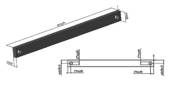
The following are dimensions and properties for the Link3 component.
| Radius of holes (radh) = 6mm |
| Width of rectangular rod (width) = 25mm |
| Thickness of rectangular rod (thick) = 10mm |
| Length of rectangular rod (length) = 300mm + 4*Radius of holes = 324mm |
| Young's modulus for rod = 7.22 x 10⁴ MPa |
| Poisson's ratio for rod = 0.34 |
| Density of rod = 2.4 x 10⁻⁹ tons/mm3 |
| Young's modulus for beams = 2.1 x 10⁵ MPa |
| Poisson's ratio for beams = 0.3 |
| Density of beams = 0.1 x 10⁻⁹ tons/mm3 |
/BATCH,list
/FILNAME,adamsout  ! Define jobname
/TITLE,Export flexible component to Adams
!
/PREP7             ! Enter preprocessor
!
! Define Parameters of rectangular rod
radh=6             ! Radius of the holes in the rod
thick=10           ! Rod thickness
width=25           ! Rod width
length=300+4*radh  ! Rod length
! Build geometry
RECTNG,0,length,0,width
CYL4,2*radh,width/2,radh
CYL4,length-2*radh,width/2,radh
ASBA,1,2
ASBA,4,3
VEXT,1, , ,0,0,thick
!
ET,1,SOLID185,,3   ! Define SOLID185 as element type 1
ET,2,BEAM188,,,3   ! Define BEAM188 as element type 2
!
MP,EX,1,7.22e4     ! Material of the rectangular rod
MP,PRXY,1,0.34
MP,DENS,1,2.4e-9
!
MP,EX,2,2.1e5      ! Material of the beams used for the spiderweb
MP,PRXY,2,0.3
MP,DENS,2,0.1e-9
!
SECTYPE,1,BEAM,ASEC
SECDATA,78.528,490.67,,490.67,,10,,,0.85716,0.85716
!
TYPE,1             ! Set element type attribute pointer to 1
MAT,1              ! Set material attribute pointer to 1
ESIZE,thick/3,0,   ! Define global element size
VSWEEP,1           ! Mesh rod
!
! Define interface points: numbers must be higher than highest
! node number already defined
N,100000,2*radh,width/2,thick/2          ! Define interface point 1
N,100001,length-2*radh,width/2,thick/2   ! Define interface point 2
!
NWPAVE,100000      ! Set working plane to interface point 1
WPSTYL,,,,,,1      ! Set working plane type to cylindrical
CSYS,4             ! Activate working plane
NSEL,S,LOC,X,radh  ! Select nodes on cylindrical hole
NSEL,A,,,100000    ! Also select interface node
!
! Generate spiderweb of beams
*GET,nmin,node,,num,min
*GET,nnum,node,,count
*SET,jj,0
TYPE,2
MAT,2
REAL,1
*DO,jj,1,nnum-2
	E,100000,nmin
	NSEL,u,,,nmin
	*GET,nmin,node,,num,min
*ENDDO
!
ALLS
!
NWPAVE,100001      ! Set working plane to interface point 2
WPSTYL,,,,,,1      ! Set working plane type to cylindrical
CSYS,4             ! Activate working plane
NSEL,S,LOC,X,radh  ! Select nodes on cylindrical hole
NSEL,A,,,100001    ! Also select interface node
!
! Generate spiderweb of beams
*GET,nmin,node,,num,min
*GET,nnum,node,,count
*SET,jj,0
TYPE,2
MAT,2
REAL,1
*DO,jj,1,nnum-2
	E,100001,nmin
	NSEL,u,,,nmin
	*GET,nmin,node,,num,min
*ENDDO
!
ALLS
!
/UNITS,MPA                       ! Define units used: millimeter
                                 ! megagram, second, newton
SAVE                             ! Save database
NSEL,s,,,100000,100001           ! Select interface points
Adams,20,1                       ! Start Adams macro,
! adamsout.mnf is written
FINISH
/EXIT,nosave
At this point you may import the adamsout.mnf file into your Adams model and perform a rigid-body dynamics simulation. The Adams model should consist of the components shown in Figure 4: Linkage Assembly. After the simulation is done, export the loads acting on the Link3 component at five arbitrary “—`time steps. Name the load file loads.lod.
Once you have exported the load file, you can perform a stress analysis for Link3 in Mechanical APDL using the command input shown below.
RESUME,adamsout,db      ! Resume model
/FILNAM,adamsin         ! Change jobname
/TITLE,Import loads from Adams	    ! Change title
!
WSPRINGS                ! Create weak springs
!
! Enter Solution and solve all load steps
/SOLU
/INPUT,loads,lod        ! Read in 5 load steps written by Adams
*DO,i,1,5               ! Use a do loop to solve each load step
  LSREAD,i              ! Read in load step
  IRLF,1	                ! Activate inertia relief
  SOLVE                 ! Solve current load step
*ENDDO
!
/POST1                  ! Enter the general postprocesser
! Write deformation and equivalent stress to graphics file
/VIEW,1,1,1,1
/AUTO,1
EPLOT
/TYPE,1,4
/SHOW,
EPLOT
*DO,i,1,5
  SET,i
  PLNSOL,u,sum
  PLNSOL,s,eqv
*ENDDO
/SHOW,term
FINISH
/EXIT,nosave