For a structure spinning about an axis Δ, if a rotation about an axis perpendicular to Δ (a precession motion) is applied to the structure, a reaction moment appears. That reaction is the gyroscopic moment. Its axis is perpendicular to both the spin axis Δ and the precession axis.

In finite element modeling, the resulting gyroscopic matrix, [G], couples degrees of freedom that are on planes perpendicular to the spin axis. It is skew symmetric.

When a rotating structure vibrates at its resonant frequency, points on the spin axis undergo an orbital motion, called whirling. Whirl motion can be a forward whirl (FW) if it is in the same direction as the rotational velocity or backward whirl (BW) if it is in the opposite direction.

In the most general case, the steady-state trajectory of a node located on the spin axis, also called orbit, is an ellipse. Its characteristics are described below.

In a local coordinate system xyz where x is the spin axis, the ellipse at node I is defined by semi-major axis A, semi-minor axis B, and phase ψ (PSI), as shown:

Figure 2.1: Elliptical Orbit

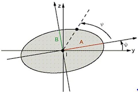
Angle ϕ (PHI) defines the initial position of the node (at t = 0). To compare the phases of two nodes of the structure, you can examine the sum ψ + ϕ.

Values YMAX and ZMAX are the maximum displacements along y and z axes, respectively.

Self-excited vibrations in a rotating structure cause an increase of the vibration amplitude over time such as shown below.

Figure 2.2: Instability

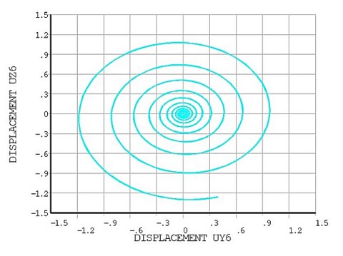
Such instabilities, if unchecked, can result in equipment damage.

The most common sources of instability are:

The critical speed is the rotational speed that corresponds to the structure's resonance frequency (or frequencies). A critical speed appears when the natural frequency is equal to the excitation frequency. The excitation may come from unbalance that is synchronous with the rotational velocity or from any asynchronous excitation.

Critical speeds can be determined by performing a Campbell diagram analysis, where the intersection points between the frequency curves and the excitation line are calculated.

Critical speeds can also be determined directly by solving a new eigenproblem, as follows. First, the case of a single rotor is detailed, then the more general case of multiple rotating and/or stationary parts.

 

2.3.5.1. Direct Critical Speeds Calculation for a Single Rotor

For an undamped rotor, the dynamics equation (Equation 1–1) is rewritten as:

(2–1)

Where [G₁] is the gyroscopic matrix corresponding to a unit rotational velocity ω.

The solution is sought in the form:

(2–2)

Where {Φ} is the mode shape and is the natural frequency.

The critical speeds are natural frequencies that are proportional to the rotational velocity.

The proportionality ratio is defined as:

(2–3)

If the excitation is synchronous (for example, unbalanced excitation), the proportionality ratio is equal to 1.0.

Replacing Equation 2–2 and Equation 2–3 into Equation 2–1 leads to the new eigenproblem:

(2–4)

Where:

(2–5)

This problem can be solved using the unsymmetric eigensolver (MODOPT,UNSYM) along with the APDLMath command *EIGEN. See Eigenvalue and Eigenvector Extraction for more details about MAPDL eigensolvers.

 

2.3.5.2. Direct Critical Speeds Calculation for Multiple Rotating and/or Stationary Parts

For an undamped multi-rotor system with stationary parts, the dynamics equation (Equation 1–1) is rewritten as:

(2–6)

where:

= total number of rotating and stationary parts

= unit gyroscopic matrix of the ith part. If the ith part is stationary, is zero.

= the rotational velocity of the ith part. If the ith part is stationary, is zero.

Assuming the first part is rotating, and taking it as the reference rotor (), rotating parts' spins are expressed as:

(2–7)

where:

= relative spin rates of the ith part. Note that for the reference rotor and . For stationary parts, .

Replacing Equation 2–7, Equation 2–3, and Equation 2–2 in Equation 2–6, a new eigenproblem is obtained:

(2–8)

where:

This problem can be solved using the damped eigensolver (MODOPT,DAMP) along with the APDLMath command *EIGEN. See Eigenvalue and Eigenvector Extraction for more details about MAPDL eigensolvers.

When designing a rotor, it is important to understand the effect of the bearing stiffness on the critical speeds. The critical speed map can be used to show the evolution of the critical speeds of the rotor with respect to the bearings stiffness.

To directly generate this map, the eigenproblem defined in Equation 2–4 is solved for different values of bearing stiffness. In this case, the model is considered undamped with identical bearings. See example in Example: Critical Speed Map Generation.