The model is a simply supported shaft. A rigid disk is located at 1/3 of its length. A bearing is located at 2/3 of its length. The rotational velocity varies with a constant slope from zero at t = 0 to 5000 RPM at t = 4 s.
The geometric properties of the shaft are as follows:
| Length: 0.4 m |
| Radius: 0.01 m |
The inertia properties of the disk are:
| Mass = 16.47 kg |
| Inertia (XX,YY) = 9.47e-2 kg·m2 |
| Inertia (ZZ) = 0.1861 kg·m2 |
The material properties for this analysis are as follows:
| Young's modulus (E) = 2.0e+11 N/m2 |
| Poisson's ratio (υ) = 0.3 |
| Density = 7800 kg/m3 |
The mass unbalance (0.1 g) is located on the disk at a distance of 0.15 m from the center line of the shaft. The mass unbalance transient forces are input using table array parameters. See Mass Unbalance Transient Forces in the Theory Reference for details of the equations. Note that the unbalance phase is 90 degrees in this example.
/prep7
! ** parameters
length = 0.4
ro_shaft = 0.01
ro_disk = 0.15
md = 16.47
id = 9.427e-2
ip = 0.1861
kxx = 2.0e+5
kyy = 5.0e+5
beta = 2.e-4
! ** material = steel
mp,ex,1,2.0e+11
mp,nuxy,1,.3
mp,dens,1,7800
! ** elements types
et,1,188
sect,1,beam,csolid
secdata,ro_shaft,20
et,2,21
r,2,md,md,md,id,id,ip
et,3,14,,1
r,3,kxx,beta*kxx
et,4,14,,2
r,4,kyy,beta*kyy
! ** shaft
type,1
secn,1
mat,1
k,1
k,2,,,length
l,1,2
lesize,1,,,9
lmesh,all
! ** disk
type,2
real,2
e,5
! ** bearing
n,21,-0.05,,2*length/3
type,3
real,3
e,8,21
type,4
real,4
e,8,21
! ** constraints
dk,1,ux,,,,uy
dk,2,ux,,,,uy
d,all,uz
d,all,rotz
d,21,all
finish
! ** transient tabular force (unbalance)
pi = acos(-1)
spin = 5000*pi/30
tinc = 0.5e-3
tend = 4
spindot = spin/tend
nbp = nint(tend/tinc) + 1
unb = 1.e-4
f0 = unb*ro_disk
*dim,spinTab,table,nbp,,,TIME
*dim,rotTab, table,nbp,,,TIME
*dim,fxTab, table,nbp,,,TIME
*dim,fyTab, table,nbp,,,TIME
*vfill,spinTab(1,0),ramp,0,tinc
*vfill,rotTab(1,0), ramp,0,tinc
*vfill,fxTab(1,0), ramp,0,tinc
*vfill,fyTab(1,0), ramp,0,tinc
tt = 0
*do,iloop,1,nbp
spinVal = spindot*tt ! omega use to compute coriolis force and omega^2
spinTab(iloop,1) = spinVal ! table of omega vs time
spin2 = spinVal**2 ! omega^2 used to compute centrifugal force
rotVal = spindot*tt**2/2 ! total rotation in radians
rotTab(iloop,1) = rotVal ! table of rotation vs time
sinr = sin(rotVal) ! direction of force based on rotVal
cosr = cos(rotVal)
fxTab(iloop,1)= f0*(-spin2*sinr + spindot*cosr) ! centrifugal force plus
! tangential force due to
fyTab(iloop,1)= f0*( spin2*cosr + spindot*sinr) ! rotation acceleration
tt = tt + tinc ! time used to compute omega
! and rotation
*enddo
fini
! ** transient analysis
/solu
antype,transient
time,tend
deltim,tinc,tinc/10,tinc*10
kbc,0
coriolis,on,,,on
omega,,,spin
f,5,fx,%fxTab%
f,5,fy,%fyTab%
outres,all,all
solve
fini
! ** generate response graphs
/post26
nsol,2,5,U,X,UXdisk
prod,3,2,2
nsol,4,5,U,Y,UYdisk
prod,5,4,4
add,6,3,5
sqrt,7,6,,,Ampl_At_Disk
/axlab,y,Displacement (m)
/show,JPEG
plvar,7
EXTREME,7
/show,CLOSE
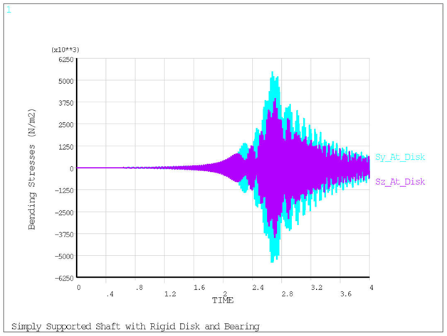
esol,8,4,5,smisc,32,Sy_At_Disk
esol,9,4,5,smisc,34,Sz_At_Disk
/axlab,y,Bending Stresses (N/m2)
/show,JPEG
plvar,8,9
EXTREME,8,9
/show,CLOSE
Figure 7.5: Transient Response – Displacement vs. Time shows displacement vs. time.
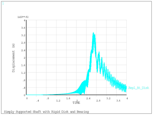
Figure 7.6: Transient Response - Bending Stress vs. Time shows bending stress vs. time.