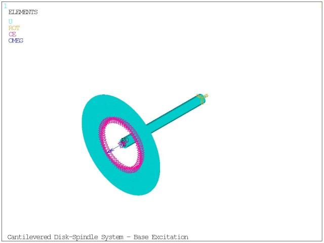
The model, a cantilevered disk-spindle system, is shown in Figure 7.1: Cantilevered Disk Spindle. The disk is fixed to the spindle with a rigid clamp and is rotating at 0.75*50 Hz. The base excitation is a harmonic force along the negative Y direction, with a frequency of up to 500 Hz.
The geometric properties of the disk are as follows:
| Thickness: 1.0 mm |
| Inner radius: 0.1016 m |
| Outer radius: 0.2032 m |
The geometric properties of the shaft are as follows:
| Length: 0.4064 m |
| Radius: 0.0191 m |
The clamp is modeled with constraint equations. The inertia properties of the clamp are:
| Mass = 6.8748 kg |
| Inertia (XX,YY) = 0.0282 kg.m2 |
| Inertia (ZZ) = 0.0355 kg.m2 |
The material properties for this analysis are as follows
| Young's modulus (E) = 2.04e+11 N/m2 |
| Poisson's ratio (υ) = 0.28 |
| Density = 8030 kg/m3 |
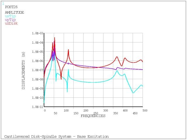
! ** parameters
pi = acos(-1)
xb = 0.1016
xa = 0.2032
zh = 1.0e-3
rs = 0.0191
ls = 0.4064
d1 = 0.0132
spin = 50*2*pi*0.75
fexcit = 500

/prep7

! ** material
mp,ex,,2.04e+11
mp,nuxy,,.28
mp,dens,,8030.

! ** spindle
et,1,188
sectype,1,beam,csolid
secd,rs,30
type,1
secn,1
k,1,,,-ls-d1
k,2,,,-d1
l,1,2
lesize,1,,,5
lmesh,all

! ** disk
et,2,181
sectype,2,shell
secd,zh
type,2
secn,2
esize,0.01
cyl4,,,xb,0,xa,360
amesh,all

! ** clamp between disk and spindle
et,3,21
r,3,6.8748,6.8748,6.8748,0.0282,0.0282,0.0355
type,3
real,3
n,
ncent = node(0,0,0)
e,ncent
cerig,ncent,node(0,0,-d1),all
csys,1
nsel,,loc,x,xb
nsel,a,node,,ncent
cerig,ncent,all,all
allsel
csys,0

! ** constraints = clamp free end
nsel,,node,,node(0,0,-ls-d1)
d,all,all,0.0
allsel
fini

! *** modal analysis in rotation
/solu
antype,modal
modopt,qrdamp,30
mxpand,30
betad,1.e-5
coriolis,on,,,on
omega,,,spin
acel,,-1	!! generate load vector
solve
fini

! *** harmonic analysis in rotation
/solu
antype,harmonic
hropt,msup,30
outres,all,none
outres,nsol,all
acel,0,0,0
kbc,0
harfrq,,fexcit
nsubst,500
lvscale,1.0      !! use load vector
solve
fini

! *** expansion
/solu
expass,on
numexp,all
solve

! *** generate response plot
/post26
nsol,2,node(0,0,0),U,X,uxTip
nsol,3,node(0,0,0),U,Y,uyTip
nsol,4,node(0,xa,0),U,Z,uzDisk
/gropt,logy,on
/axlab,x,FREQUENCIES
/axlab,y,DISPLACEMENTS (m)
/show,JPEG
plvar,2,3,4
EXTREM,2,4,1
/show,CLOSE
Figure 7.2: Output for the Cantilevered Disk Spindle shows the graph of displacement versus frequency.