


Several interpolation algorithms are available for use with supported material data tables (TB).
Simple linear interpolation is the default for 1D and 2D grid data. To obtain meaningful results for multidimensional non-grid data, it is necessary to use one of the multidimensional interpolation algorithms.
You can select an interpolation algorithm or switch between algorithms (TBIN).
The following topics for interpolation algorithms are available:
Simple linear interpolation can be used for one- and two-dimensional grid data:
To demonstrate the interpolation of data in a sparsely defined grid, consider the results of a two-dimensional interpolation at a temperature of 100 and a sliding distance of 0.40. In this case, the program performs only a one-dimensional interpolation because the defined temperature value (100) lies directly on the defined grid field. For this case, the program obtains a friction coefficient value of 0.45 based on the following calculations:


Substituting the tabular values
x = 0.4, x0 = 0.2, x1 = 0.5 y0 = 0.35 y1 = 0.5
Substituting these values into Equation (2):

Equation (3)
and solving for the interpolated values using Equation (1), we obtain

Equation (4)
Two-dimensional interpolation requires data provided in the proper order. If UF01 and TEMP are the two field variables, for example, input the data in the following format:
| UF01 = 100 | UF01 = 200 | UF01 = 300 | UF01 = 400 | |
| TEMP = 0 | 1 | 2 | 3 | 4 |
| TEMP = 10 | 5 | 6 | ||
| TEMP = 20 | 7 | 8 | 9 |
If TBFIELD for TEMP is issued first, all data points with TEMP held constant and UF01 varying are issued. Then TEMP is modified again and data points with UF01 changing are issued.
Consider the case where a true two-dimensional interpolation is required at a temperature of 180 and a sliding distance of 0.40. The program performs three different linear interpolations to determine the property value within the grid. When performing two-dimensional interpolation, the program always interpolates first along the two relevant rows of the grid (Temperature in this case), then between the rows.
In this example, the program performs the first interpolation at a temperature of 100 and a sliding distance of 0.4, yielding the result of 0.45 (as shown in Equation (4)).
The program performs the second interpolation for a temperature of 200 and a sliding distance of 0.4. In this case, we find that
x = 0.4, x0 = 0.2, x1 = 0.5 y0 = 0.2 y1 = 0.14
Substituting these values into Equation (2):

Equation (5)
and solving for the interpolated values using Equation (1), we obtain

Equation (6)
Finally, the program performs a third interpolation between the temperature value of 100 and 200 at a sliding distance of 0.4.
t = 180, t0 = 100, t1 = 200 y0 = 0.45 y1 = 0.16
Substituting these values into Equation (2):

Equation (7)
and solving for the interpolated values using Equation (1), we obtain

Equation (8)
Use the linear-multivariate algorithm to perform interpolation when two or more field variables are input.
Unlike simple linear interpolation, you can input a random collection of data points where the material property was experimentally evaluated. It is not necessary to input data in any specific grid format (although you can still do so), but you must provide enough data to cover the region where you intend to interpolate.
Because the data is a random sampling, the algorithm creates an
n-dimensional rectangular bounding box, and the
queries outside of the bounding box are projected to fall on the surface or edge of
the bounding box. The algorithm performs the projection by calculating a normal to
each axis until it finds a position within the bounding box.
In the following figure, the stars represent the data points input that you provide, and the blue stars represent queries outside of the bounding box:
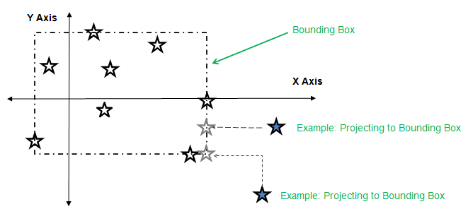
The figure shows how the data points are projected first in one dimension and then in the second dimension. This method was extrapolated and implemented for multiple dimensions.
Nonlinear interpolation can produce slightly different results from that of linear interpolation.
For material data tables that use TBPT-based input (such as TB,PLASTIC), stresses are first evaluated at the neighboring strain values provided in the TBPT input using the specified multidimensional interpolation algorithm, then linearly interpolated between the neighboring values to maintain the stress strain data C0.
Linear-multivariate is an interpolation algorithm that uses points near the
query location to perform the interpolation process. The algorithm generates an
n-dimension mesh (simplices) using Delaunay
triangulation. It uses that mesh to select an
n-dimensional element, and the values at the nodes of
the elements, to perform a linear interpolation.
The linear-multivariate algorithm is recommended for parameter spaces of Order 3 and above, or when the data is not a standard 2D grid. It is highly accurate when given a sufficient distribution of points. (More data points result in greater accuracy.)
The linear-multivariate algorithm is also capable of projecting points to the convex hull generated prior to the interpolation process, as shown in Example 9.6: Projecting to a Convex Hull.
When using linear-multivariate interpolation, examine the input and the
interpolated values (*GET) before
applying the algorithm to the solution. (See *GET General Items, Entity = TBTYPE in the Command Reference and Evaluating Interpolation Algorithm Results.) The
following example cases indicate the necessity of performing an interpolation
study for complex data:
Example 9.3: Linear-Multivariate Interpolation Using Four Points
In some cases, such as a perfect grid, the triangulation may not be unique. In this 2D example with the given four points, the generated mesh can take either of these forms:
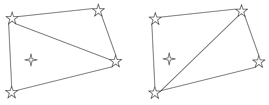
If all four points are not in a plane, the linearly interpolated value is generated either from the bottom three points or from the leftmost three points, depending on how the mesh was generated internally. Enter enough points to ensure that any meshing changes do not affect the results.
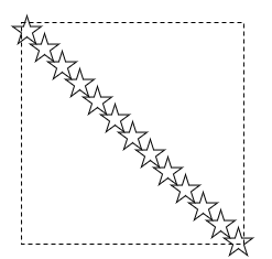
Example 9.4: Dimensionality of Data
Linear-multivariate interpolation cannot handle data where the dimensionality of the data points is higher than the dimensionality of the point cloud.
For example, with 2D data, the algorithm cannot handle cases where all points lie in a single line. You must therefore either transform the data to a single dimension or populate the 2D data with additional data points to enable the algorithm to create a 2D mesh.
Likewise, avoid using this algorithm if the data points are 3D but span only a surface (a dimension less than the dimension of the point) rather than a 3D volume.
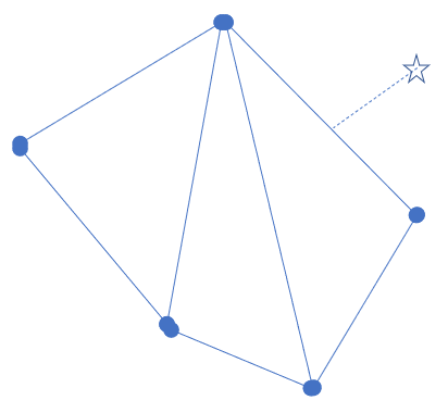
Example 9.5: Query Points Outside the Convex Hull of Input Data Points
Here is an example of a situation when the query point (blue star) is specified outside the convex hull of the specified data points but inside the bounding box:
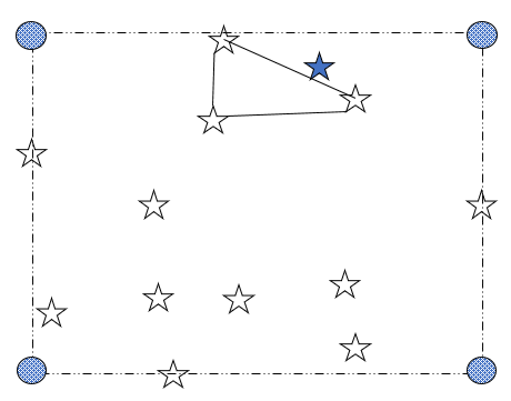
By default, an error occurs in such cases (because the data from the nearest element will need to be extrapolated to obtain a result). To avoid this situation:
Define the corner points (blue circles) of the bounding box, or
Issue TBIN,,EXTR,PHULL. (See Example 9.6: Projecting to a Convex Hull.)
Example 9.6: Projecting to a Convex Hull
The query point is projected in the normal direction to a convex hull for a two-dimensional input (enabled via TBIN,,EXTR,PHULL):
If the field variable range differs in the various dimensions, Ansys, Inc. recommends using normalization (TBIN,NORM), enabled by default. For example, use normalization when temperatures range from 100 to 300 and UF01 (such as material fraction) ranges from 1e-5 to 3e-5.
For more information about the linear-multivariate algorithm, see Linear Multivariate Interpolation in the ACP User's Guide.
The following example input shows how to input and evaluate the interpolation algorithm via *GET:
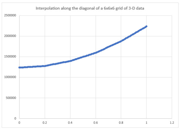
! Example: evaluating interpolation of material data tables
/prep7

! Use a six X six X six grid
xpts=6
ypts=6
zpts=6

! 3D Grid is unnecessary. The grid below is created for demonstration
! purposes only.

! Setting up a TB,ELAS property with linear-multivariate interpolation algorithm
tb,elas,1
*DO,x,1,xpts,1
*DO,y,1,ypts,1
*DO,z,1,zpts,1
xloc=(x-1)/(xpts-1)
yloc=(y-1)/(ypts-1)
zloc=(z-1)/(zpts-1)
tbfield,xcor,xloc
tbfield,ycor,yloc
tbfield,zcor,zloc
E=(1+xloc**2+yloc**2+zloc**2)*1e6
tbdat,,E,0.0
*ENDDO
*ENDDO
*ENDDO
tbin,algo,lmul

*dim,ucalc,,101
*dim,zcalc1,,101

! Issue the *GET command to evaluate the value on
! a line across the data
*DO,x,1,101,1
myval=(x-1)/100
ucalc(x)=myval
*get,velas,elas,1,tbev,1,1,3,0.33,0.33,myval
zcalc1(x)=velas
*ENDDO

*stat,ucalc,1,101
*stat,zcalc1,1,101
finish
Simple linear interpolation is supported for all material data tables.
Linear-multivariate interpolation is supported for these material data tables:
| Material Model |
TB,Lab
Value |
|---|---|
| Coefficient of thermal expansion | CTE |
| Mass density | DENS |
| Elasticity | ELASTIC |
| Hyperelasticity | HYPER |
| Nonlinear plasticity | PLAS |
| Porous media | PM |